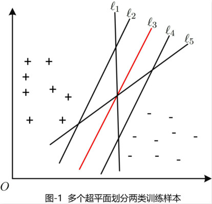
给定系统模型
\begin{align}
\boldsymbol{y}=g(\boldsymbol{x})
\end{align}
其中$\boldsymbol{x}\in \mathbb{R}^M$是目标信号,其随机性由先验概率$p(\boldsymbol{x})$刻画;$\boldsymbol{y}\in \mathbb{R}^N$是观测信号;函数$g(\cdot)$表示从$N$维空间到$M$维空间的映射,即$g(\cdot):\mathbb{R}^N\rightarrow \mathbb{R}^M$。在信号重构理论的研究对象中,映射$g(\cdot)$以及先验概率$p(\boldsymbol{x})$均给定,我们需要从观测信号$\boldsymbol{y}$中恢复出目标信号$\boldsymbol{x}$来。映射函数$g(\cdot)$可以是线性的,如线性高斯模型$g(\boldsymbol{x})=\boldsymbol{Hx}+\boldsymbol{w}$,也可以是非线性函数,如ADC量化模型$g(\boldsymbol{x})=Q(\boldsymbol{Hx}+\boldsymbol{w})$,其中$Q(\cdot)$表示均匀量化函数。
贝叶斯估计理论是众多信号重构算法中的一类算法。贝叶斯估计器被定义为使得如下贝叶斯风险函数最小
\begin{align}
\hat{\boldsymbol{x} }_{\text{Bayse} }
&=\underset{\hat{\boldsymbol{x} } }{\arg \min}\ \mathbb{E}_{\boldsymbol{x},\boldsymbol{y} }\left[\mathcal{C}(\boldsymbol{\epsilon})\right]\\
&=\underset{\hat{\boldsymbol{x} } }{\arg \min} \int_{\boldsymbol{y} }\left[\int_{\boldsymbol{x} }\mathcal{C}(\boldsymbol{\epsilon})p(\boldsymbol{x}|\boldsymbol{y})\text{d}\boldsymbol{x}\right]p(\boldsymbol{y})\text{d}\boldsymbol{y}\\
&=\underset{\hat{\boldsymbol{x} } }{\arg \min} \int_{\boldsymbol{x} }\mathcal{C}(\boldsymbol{\epsilon})p(\boldsymbol{x}|\boldsymbol{y})\text{d}\boldsymbol{x}
\end{align}
其中$\mathcal{C}(\boldsymbol{\epsilon})$表示代价函数,$\boldsymbol{\epsilon}=\hat{\boldsymbol{x} }-\boldsymbol{x}$。 为了简化符号,定义
\begin{align}
g(\epsilon)\overset{\triangle}{=}\int_{\boldsymbol{x} }\mathcal{C}(\epsilon) p(\boldsymbol{x}|\boldsymbol{y})\text{d}\boldsymbol{x}
\end{align}
换言之,贝叶斯估计器是通过最小化$g(\boldsymbol{\epsilon})$得到。为了得到贝叶斯估计器的具体表达式,我们需要进一步确定代价函数的具体形式。特别需要注意的是,代价函数的选择应该数学上尽量简单出发。满足此要求的代价函数,如图所示,有二次误差型(quadratic error)、成功-失败型(hit-or-miss error)、绝对误差型(absolute error)。
当选择代价函数为二次误差型函数时,有
\begin{align}
g(\boldsymbol{\epsilon})=\int_{\boldsymbol{x} } |\hat{\boldsymbol{x} }-\boldsymbol{x}|^2 p(\boldsymbol{x}|\boldsymbol{y})\text{d}\boldsymbol{x}
\end{align}
上式求$\hat{\boldsymbol{x} }$求偏导,并设偏导为0,有
\begin{align}
\int (\hat{\boldsymbol{x} }-\boldsymbol{x}) p(\boldsymbol{x}|\boldsymbol{y})\text{d}\boldsymbol{x}=0
\end{align}
整理为
\begin{align}
\hat{\boldsymbol{x} }=\mathbb{E}\left[\boldsymbol{x}|\boldsymbol{y}\right]=\int_{\boldsymbol{x} }\boldsymbol{x} p(\boldsymbol{x}|\boldsymbol{y})\text{d}\boldsymbol{x}
\end{align}
由于该估计器使得均方误差最小,因此被称之为最小均方误差估计。此外,该估计器的表达形式为后验概率的均值,因此也被称为后验均值估计。
当选择代价函数为“成功-失败”型代价函数(图b)时,有
\begin{align}
g(\boldsymbol{\epsilon})
&=\lim_{\kappa\rightarrow 0} \left[
\int_{\hat{\boldsymbol{x} }+\kappa}^{+\infty}p(\boldsymbol{x}|\boldsymbol{y})\text{d}\boldsymbol{x}+\int_{-\infty}^{\hat{\boldsymbol{x} }-\kappa}p(\boldsymbol{x}|\boldsymbol{y})\text{d}\boldsymbol{x}
\right]\\
&=1-\lim_{\kappa\rightarrow 0}\int_{\hat{\boldsymbol{x} }-\kappa}^{\hat{\boldsymbol{x} }+\kappa}p(\boldsymbol{x}|\boldsymbol{y})\text{d}\boldsymbol{x}
\end{align}
为了使得$g(\boldsymbol{\epsilon})$最小,需使得$\lim_{\kappa\rightarrow 0}\int_{\hat{\boldsymbol{x} }-\kappa}^{\hat{\boldsymbol{x} }+\kappa}p(\boldsymbol{x}|\boldsymbol{y})$最大,因此选择后验概率的最大值点作为估计器。由于该估计器选择后验概率的最大值点作为估计器,因此被称为最大后验概率估计,即
\begin{align}
\hat{\boldsymbol{x} }=\underset{\boldsymbol{x} }{\arg \max} \ p(\boldsymbol{x}|\boldsymbol{y})
\end{align}
若选择绝对误差型误差函数时,此时
\begin{align}
g(\boldsymbol{\epsilon})
&=\int |\boldsymbol{x}-\hat{\boldsymbol{x} }| p(\boldsymbol{x}|\boldsymbol{y})\text{d}\boldsymbol{x}\\
&=\int_{\hat{\boldsymbol{x} } }^{+\infty} (\boldsymbol{x}-\hat{\boldsymbol{x} }) p(\boldsymbol{x}|\boldsymbol{y})\text{d}\boldsymbol{x}+\int_{-\infty}^{\hat{\boldsymbol{x} } } (\hat{\boldsymbol{x} }-\boldsymbol{x})p(\boldsymbol{x}|\boldsymbol{y})\text{d}\boldsymbol{x}
\end{align}
上式对$\hat{\boldsymbol{x} }$求偏导,并令其为0,得到
\begin{align}
\int_{-\infty}^{\hat{\boldsymbol{x} } }p(\boldsymbol{x}|\boldsymbol{y})\text{d}\boldsymbol{x}=\int_{\hat{\boldsymbol{x} } }^{+\infty}p(\boldsymbol{x}|\boldsymbol{y})\text{d}\boldsymbol{x}
\end{align}
此时估计器$\hat{\boldsymbol{x} }$为后验概率$p(\boldsymbol{x}|\boldsymbol{y})$的中值点,即$\text{Pr}(\boldsymbol{x}\leq \hat{\boldsymbol{x} })=\frac{1}{2}$。
通常来说,如下图所示后验概率的均值点、最大值点、中值点各不一样。特别地,若后验概率为高斯分布时,三点重合。
事实上,后验概率的中值点通常难以得到,除了某些特殊分布,如高斯分布,因此,常用的贝叶斯估计器主要指最小均方误差估计和最大后验概率估计。
]]>We consider mixtrue Gaussian distribution
\begin{align}
p(h)=\sum_{k=1}^K \rho_k \mathcal{N}_c(h|0,\sigma_k^2)
\end{align}
Followings are two conditions of mixture Gaussian distribution
The mean and variance of distribution
\begin{align}
&\frac{p(h)\mathcal{N}_c(h|m,v)}{\int p(h)\mathcal{N}_c(h|m,v) \text{d}h}\\
=&\frac{\sum_{k=1}^K \rho_k\mathcal{N}_c(h|0,\sigma_k^2)\mathcal{N}_c(h|m,v)}{\int \sum_{k=1}^K \rho_k\mathcal{N}_c(h|0,\sigma_k^2)\mathcal{N}_c(h|m,v) \text{d}h}\\
=&\frac{\sum_{k=1}^K \rho_k\mathcal{N}_c\left(m|0,\sigma_k^2+v\right)\mathcal{N}_c\left(h|\frac{m\sigma_k^2}{\sigma_k^2+v},\frac{\sigma_k^2v}{\sigma_k^2+v}\right)}
{\sum_{k=1}^K \rho_k\mathcal{N}_c\left(m|0,\sigma_k^2+v\right)}
\end{align}
are given
\begin{align}
f_a(h|m,v)
&\overset{\triangle}{=}\mathbb{E}[h|m,v]\\
&=\frac{\sum_{k=1}^K\rho_k \frac{m\sigma_k^2}{\sigma_k^2+v}\mathcal{N}_c\left(m|0,\sigma_k^2+v\right)}{\sum_{k=1}^K \rho_k \mathcal{N}_c(m|0,\sigma_k^2+v)}\\
f_b(h|m,v)&\overset{\triangle}{=}\mathbb{E}[|h|^2|m,v]\\
&=\frac{\sum_{k=1}^K\rho_k \left[\frac{\sigma_k^2v}{\sigma_k^2+v}+\left(\frac{m\sigma_k^2}{\sigma_k^2+v}\right)^2\right]\mathcal{N}_c\left(m|0,\sigma_k^2+v\right)}{\sum_{k=1}^K \rho_k \mathcal{N}_c(m|0,\sigma_k^2+v)}\\
&=\frac{\sum_{k=1}^K\rho_k \left[\frac{\sigma_k^2v(\sigma_k^2+v)+|m|^2\sigma_k^4}{(\sigma_k^2+v)^2}\right]\mathcal{N}_c\left(m|0,\sigma_k^2+v\right)}{\sum_{k=1}^K \rho_k \mathcal{N}_c(m|0,\sigma_k^2+v)}\\
\end{align}
where the expectation is over $\frac{p(h)\mathcal{N}_c(h|m,v)}{\int p(h)\mathcal{N}_c(h|m,v) \text{d}h}$. Based on above, we get
\begin{align}
f_c(h|m,v)&\overset{\triangle}{=}\text{Var}[h|m,v]\\
&=f_b(h|m,v)-|f_a(h|m,v)|^2
\end{align}
Given the Gaussian mixture distribution
\begin{align}
p(h)=\sum_{k=1}^K \rho_k \mathcal{N}_c\left(h|0,\sigma_k^2\right)
\end{align}
and equivalent scalar channel
\begin{align}
m=h+n \sim \mathcal{N}_c(n|0,v)
\end{align}
the distribution of $m$ is then expressed by
\begin{align}
p(m)=\sum_{k=1}^K \rho_k\mathcal{N}_c(m|0,v+\sigma_k^2)
\end{align}
$proof$:
$\underline{\text{Step 1} }$: Assume $X\sim \mathcal{N}(x|a,A)$ and $Y\sim \mathcal{N}(y|b,B)$. Define $Z=X+Y$, then its distribution is obtained by convolution formula
\begin{align}
p(z)
&=\int_{-\infty}^{+\infty} p_X(x)p_Y(z-x)\text{d}x\\
&=\int_{-\infty}^{+\infty}\mathcal{N}(x|a,A)\mathcal{N}(z-x|b,B)\text{d}x\\
&=\int_{-\infty}^{+\infty}\mathcal{N}(x|a,A)\mathcal{N}(x|b-z,B)\text{d}x\\
&\overset{(a)}{=}\mathcal{N}(0|a-(b-z),A+B)\\
&=\mathcal{N}(z|b-a,A+B)
\end{align}
where $(a)$ holds by Gaussian product lemma.
$\underline{\text{Step 2} }$: Assume $X\sim \sum_{k=1}^K \mathcal{N}(x|a_k,A_k)$ and $Y\sim \mathcal{N}(y|b,B)$. Define $Z=X+Y$, using the convolution formula we can easy get
\begin{align}
p(z)
&=\int_{-\infty}^{+\infty}p_X(x)p_Y(z-x)\text{d}x\\
&=\int_{-\infty}^{+\infty}\sum_{k=1}^K\rho_k\mathcal{N}(x|a_k,A_k)\mathcal{N}(z-x|b,B)\text{d}x\\
&=\int_{-\infty}^{+\infty}\sum_{k=1}^K \rho_k \mathcal{N}(x|a_k,A_k)\mathcal{N}(x|b-z,B)\text{d}x\\
&=\sum_{k=1}^K \rho_k \mathcal{N}(0|a_k-(b-z),A_k+B)\\
&=\sum_{k=1}^K\rho_k\mathcal{N}(z|b-a_k,A_k+B)
\end{align}
$\underline{\text{Step 3} }$: If $a_k$ and $b$ are equal to zero, we then get
\begin{align}
p(z)=\sum_{k=1}^K \rho_k \mathcal{N}(z|0,A_k+B)
\end{align}
The MMSE of this AWGN model is given by
\begin{align}
\text{MMSE}
&=\mathbb{E}[\text{Var}[h|m,v]]\\
&=\int f_c(h|m,v)\sum_{k=1}^K\rho_k\mathcal{N}_c(m|0,\sigma_k^2+v)\text{d}m\\
&=\int \left[\frac{\sum_{k=1}^K\rho_k \left[\frac{\sigma_k^2v(\sigma_k^2+v)+|m|^2\sigma_k^4}{(\sigma_k^2+v)^2}\right]\mathcal{N}_c\left(m|0,\sigma_k^2+v\right)}{\sum_{k=1}^K \rho_k \mathcal{N}_c(m|0,\sigma_k^2+v)}-\left|\frac{\sum_{k=1}^K\rho_k \frac{m\sigma_k^2}{\sigma_k^2+v}\mathcal{N}_c\left(m|0,\sigma_k^2+v\right)}{\sum_{k=1}^K \rho_k \mathcal{N}_c(m|0,\sigma_k^2+v)}\right|^2\right]\\
&\quad \times \sum_{j=1}^K\rho_j\mathcal{N}_c(m|0,\sigma_j^2+v)\text{d}m\\
&=\sum_{k=1}^K\rho_k\frac{\sigma_k^2v+\sigma_k^4}{\sigma_k^2+v}-\int \left|\frac{\sum_{k=1}^K\rho_k \frac{m\sigma_k^2}{\sigma_k^2+v}\mathcal{N}_c\left(m|0,\sigma_k^2+v\right)}{\sum_{k=1}^K \rho_k \mathcal{N}_c(m|0,\sigma_k^2+v)}\right|^2 \sum_{j=1}^K \rho_j\mathcal{N}_c(m|0,\sigma_j^2+v)\text{d}m
\end{align}
where the inner expectation is over $\frac{p(h)\mathcal{N}_c(h|m,v)}{\int p(h)\mathcal{N}(h|m,v)\text{d}h}$ while the outer expectation is taken over $p(m)=\sum_{k=1}^K \rho_k\mathcal{N}(m|0,\sigma_k^2+v)$.
As mentioned in [1], we have introduced variational inference and its application in Bayesian linear regression. In this blog, we will introduce a variational inference perspective on expectation propagation.
In signal processing, the posterior distribution is interested. However, it is difficult to obtain since many high-dimension integral are involved. For example, we consider linear Gaussian model
\begin{align}
\mathbf{y}=\mathbf{Hx}+\mathbf{w}
\end{align} Its posterior distribution is given by
\begin{align}
p(\mathbf{x}|\mathbf{y})=\frac{p(\mathbf{y}|\mathbf{x})p(\mathbf{x})}{\int p(\mathbf{y}|\mathbf{x})p(\mathbf{x}) \text{d}\mathbf{x} }
\end{align} where $p(\mathbf{y}|\mathbf{x})=p_{\mathbf{w} }(\mathbf{y}-\mathbf{Hx})$. Unless both $p(\mathbf{y}|\mathbf{x})$ and $p(\mathbf{x})$ are Gaussian, it is difficult to easily obtain the close-form of $p(\mathbf{x}|\mathbf{y})$. Some approximations, thus, are necessary.
For that purpose, we use $q(\mathbf{x})$ to approximate the posterior distribution and applied KL-divergence to measure the difference between $q(\mathbf{x})$ and $p(\mathbf{x}|\mathbf{y})$. For simplication, we generally restrict the form of $q(\mathbf{x})$ from the distribution family $\mathcal{S}$, i.e.,
\begin{align}
q(\mathbf{x})=\underset{q(\mathbf{x})\in \mathcal{S} } {\arg \min} \ \mathcal{D}_{\text{KL} }(p||q)
\end{align} Obviously, a distribution family with excellent properties will greatly reduce the amount of computation. Luckily, the exponential family is one of those.
The exponential family over $\mathbf{x}$ parametered by $\boldsymbol{\eta}$ is defined by following form
\begin{align}
p(\mathbf{x};\boldsymbol{\eta})=h(\mathbf{x})g(\boldsymbol{\eta})\exp\left(\boldsymbol{\eta}^T\boldsymbol{u}(\mathbf{x})\right)
\end{align} where $g(\boldsymbol{\eta})$ is normalization constant
\begin{align}
g(\boldsymbol{\eta}) \left[\int h(\mathbf{x})\exp\left(\boldsymbol{\eta}^T\boldsymbol{u}(\mathbf{x})\right)\text{d}\mathbf{x}\right]=1
\end{align} Taking the gradient of both side of the above w.r.t. $\boldsymbol{\eta}$, we get
\begin{align}
\nabla g(\boldsymbol{\eta})\int h(\mathbf{x})\exp \left(\boldsymbol{\eta}^T\boldsymbol{u}(\mathbf{x})\right)\text{d}\mathbf{x}+g(\boldsymbol{\eta})\int h(\mathbf{x})\left(\boldsymbol{\eta}^T\boldsymbol{u}(\mathbf{x})\right)\boldsymbol{u}(\mathbf{x})\text{d}\mathbf{x}=0
\end{align} Rearranging above equation yields
\begin{align}
-\frac{1}{g(\boldsymbol{\eta})}\nabla g(\boldsymbol{\eta})
&=g(\boldsymbol{\eta}) \int \boldsymbol{u}(\mathbf{x})h(\mathbf{x})\exp\left(\boldsymbol{\eta}^T\boldsymbol{u}(\mathbf{x})\right)\text{d}\mathbf{x}\\
&=\frac{ \int \boldsymbol{u}(\mathbf{x})h(\mathbf{x})\exp\left(\boldsymbol{\eta}^T\boldsymbol{u}(\mathbf{x})\right)\text{d}\mathbf{x} }{ \int h(\mathbf{x})\exp\left(\boldsymbol{\eta}^T\boldsymbol{u}(\mathbf{x})\right)\text{d}\mathbf{x} }\\
&=\mathbb{E}[\boldsymbol{u}(\mathbf{x})]
\end{align} Using the fact $\nabla \log g(\boldsymbol{\eta})=\frac{1}{g(\boldsymbol{\eta})}\nabla g(\boldsymbol{\eta})$, we have
\begin{align}
-\nabla \log g(\boldsymbol{\eta})=\mathbb{E}[\boldsymbol{u}(\mathbf{x})] \quad \cdots\quad (*1)
\end{align}
For the distribution of $q(\mathbf{x})$ in variational inference, We take exponential family distribution into account
\begin{align}
q(\mathbf{x})=h(\mathbf{x})g(\boldsymbol{\eta})\exp \left(\boldsymbol{\eta}^T\boldsymbol{u}(\mathbf{x})\right)
\end{align} we then write $\mathcal{D}_{\text{KL} }(p||q)$ as
\begin{align}
\mathcal{D}_{\text{KL} }(p||q)=-\log g(\boldsymbol{\eta})-\boldsymbol{\eta}^T\mathbb{E}_{p(\mathbf{x})}[\boldsymbol{u}(\mathbf{x})]+\text{const}
\end{align} Taking the gradient of both side of above w.r.t. $\boldsymbol{\eta}$ to zero yields
\begin{align}
-\nabla \log g(\boldsymbol{\eta}) =\mathbb{E}_{p(\mathbf{x})}[\boldsymbol{u}(\mathbf{x})]
\end{align} As mentioned in $(*1)$, we then get
\begin{align}
\mathbb{E}_{q(\mathbf{x})}[\boldsymbol{u}(\mathbf{x})]=\mathbb{E}_{p(\mathbf{x})}[\boldsymbol{u}(\mathbf{x})]
\end{align} Note that if $q(\mathbf{x})$ is Gaussian $\mathcal{N}(\mathbf{x}|\boldsymbol{\mu},\mathbf{\Sigma})$, we then minimize the KL-divergence by setting $\boldsymbol{\mu}$ equal to the mean of $p(\mathbf{x})$ and $\mathbf{\Sigma}$ equal to the variance of $p(\mathbf{x})$.
We exploit this result to obtain a pratical algorithm for approximate inference. For many probability models, the joint distribution of data $\mathcal{D}=\left\{\mathbf{y}_1,\cdots,\mathbf{y}_N\right\}$ and hidden variables (may including parameters) $\boldsymbol{\theta}$ comprises a product of factors in the form
\begin{align}
p(\mathcal{D},\boldsymbol{\theta})=\prod_i f_i(\boldsymbol{\theta})
\end{align} where $f_0(\boldsymbol{\theta})=p(\boldsymbol{\theta})$ and $f_n(\boldsymbol{\theta})=p(\mathbf{y}_n|\boldsymbol{\theta}),(n\ne 0)$. The posterior distribution is given by
\begin{align}
p(\boldsymbol{\theta}|\mathcal{D})=\frac{p(\mathcal{D},\boldsymbol{\theta})}{p(\mathcal{D})}=\frac{1}{p(\mathcal{D})}\prod_{i} f_i(\boldsymbol{\theta})
\end{align} where $p(\mathcal{D})$ is partition function or evidence function.
\begin{align}
p(\mathcal{D})=\int \prod_i f_i(\boldsymbol{\theta})\text{d}\boldsymbol{\theta}
\end{align} As we determine the form of $q(\mathbf{x})$
\begin{align}
q(\boldsymbol{\theta})=\frac{1}{Z}\prod_i q_i(\boldsymbol{\theta})
\end{align} then $q(\boldsymbol{\theta})$ is updated by minimizing
\begin{align}
q_i(\boldsymbol{\theta})=\underset{q_i(\boldsymbol{\theta})}{\arg \min}\ \mathcal{D}_{\text{KL} }\left(\frac{1}{p(\mathcal{D})}\prod_{i}f_i(\boldsymbol{\theta})||\frac{1}{Z}\prod_{i}q_i(\boldsymbol{\theta})\right)
\end{align} Actually, the approximation is poor since each factor is individually approximated. To remedy this situation, expectation propagation makes a much better approximation by optimizing each factor in turn in the context of all of the remaining factors [2]. Below, we will give the detailed description of EP step-by-step.
$\underline{\text{Step 1} }$: Initialize all factors $q_i(\boldsymbol{\theta})$ from distribution family $\mathcal{S}$.
\begin{align}
q(\boldsymbol{\theta})=\frac{1}{Z}\prod_i q_i(\boldsymbol{\theta})
\end{align} $\underline{\text{Step 2} }$: Compute $q^{\backslash j}(\boldsymbol{\theta})$ denoted by
\begin{align}
q^{\backslash j}(\boldsymbol{\theta})=C\frac{q(\boldsymbol{\theta})}{q_j(\boldsymbol{\theta})}
\end{align}
where $C$ is normalization constant.
$\underline{\text{Step 3} }$: Update
\begin{align}
q^{\text{new} }(\boldsymbol{\theta})=\mathcal{D}_{\text{KL} } \left(\frac{1}{Z_j}f_j(\boldsymbol{\theta})q^{\backslash j}(\boldsymbol{\theta})||q(\boldsymbol{\theta})\right)
\end{align}
where $q^{\text{new} }(\boldsymbol{\theta})$ is the update of $q(\boldsymbol{\theta})$.
$\underline{\text{Step 4} }$: Update $q_j(\boldsymbol{\theta})$
\begin{align}
q_j(\boldsymbol{\theta})=C\frac{q^{\text{new} }(\boldsymbol{\theta})}{q^{\backslash j}(\boldsymbol{\theta})}
\end{align}
where $C$ is a normalization constant.
$\underline{\text{Step 5} }$: $\longrightarrow $ Step 2.
We consider standard linear Gaussian model (SLM)
\begin{align}
\mathbf{y}=\mathbf{Hx}+\mathbf{w}
\end{align} where $\mathbf{x}\in \mathbb{C}^N$ generated from $M$-QAM constellation with distribution $p(\mathbf{x})=\prod_{i=1}^N p(x_i)$. Passing the channel $\mathbf{H}\in \mathbb{C}^{M\times N}$ (estimated perfect beforhand) and adding the white Gaussian noise $\mathbf{w}\sim \mathcal{N}_c(\mathbf{w}|\boldsymbol{0},\sigma^2\mathbf{I})$, the final observed signal $\mathbf{y}$ is then obtained.
We aim at designing an high-efficient signal detector using EP. Based on above knowledge, we write the posterior distribution of this model as
\begin{align}
p(\mathbf{x}|\mathbf{y})
&=\frac{p(\mathbf{y}|\mathbf{x})p(\mathbf{x})}{p(\mathbf{y})}\\
&\propto p(\mathbf{y}|\mathbf{x})p(\mathbf{x})
\end{align} Notice that since $\mathbf{y}$ is given, then $p(\mathbf{y})$ is regarded as a constant. We further assume the each observed data are independent of others, i.e.,
\begin{align}
p(\mathbf{y}|\mathbf{x})=\prod_{a=1}^M p(y_a|\mathbf{x})
\end{align} $\underline{\text{Step 1} }$: Initialize $q(\mathbf{x})$, the approximation of $q(\mathbf{x})$. Since $p(\mathbf{y}|\mathbf{x})$ is Gaussian, we then approximate $p(\mathbf{x})$ by Gaussian, one of exponential family.
\begin{align}
q(\mathbf{x})=\mathcal{N}_c(\mathbf{x}|\mathbf{m},\text{Diag}(\mathbf{v}))
\end{align} Its marginal distribution is $q(x_i)=\mathcal{N}_c(x_i|m_i,v_i)$. Note that $q(x_i)$ here is $q_i(\boldsymbol{\theta})$ mentioned in section 3.
$\underline{\text{Step 2} }$: Calculate the joint distribution $q(\mathbf{x},\mathbf{y})$
\begin{align}
q(\mathbf{x},\mathbf{y})
&=q(\mathbf{x})p(\mathbf{y}|\mathbf{x})\\
&=\mathcal{N}_c(\mathbf{x}|\boldsymbol{m},\text{Diag}(\mathbf{v}))\mathcal{N}_c(\mathbf{y}|\mathbf{Hx},\sigma^2\mathbf{I})\\
&\propto \mathcal{N}_c(\mathbf{x}|\boldsymbol{m},\text{Diag}(\mathbf{v}))\mathcal{N}_c(\mathbf{x}|(\mathbf{H}^T\mathbf{H})^{-1}\mathbf{H}^H\mathbf{y},(\sigma^{-2}\mathbf{H}^T\mathbf{H})^{-1}) \\
&\propto \mathcal{N}_c(\mathbf{x}|\boldsymbol{\mu},\mathbf{\Sigma})
\end{align} where the last equaiton holds by Gaussian product lemma mentioned in [2] and following definitions
\begin{align}
\mathbf{\Sigma}&=(\sigma^{-1}\mathbf{H}^H\mathbf{H}+\text{Diag}(\mathbf{1}\oslash \mathbf{v}))^{-1}\\
\boldsymbol{\mu}&=\mathbf{\Sigma}\left(\sigma^2\mathbf{H}^H\mathbf{y}+\text{Diag}(\mathbf{m}\oslash \mathbf{v})\right)
\end{align} Here, we further abuse $\mathcal{N}_c(x_j|\mu_{j},\Sigma_{jj})$ to approximate $p(x_j,\mathbf{y})$, the marignal distribuiton of $p(\mathbf{x},\mathbf{y})$. This operation ignores the correlation of $x_j$ and $\mathbf{x}_{\backslash j}$, so we write it as $q(x_j,\mathbf{y})=\mathcal{N}_c(x_j|\mu_j,\Sigma_{jj})$.
$\underline{\text{Step 3} }$: Compute $q^{\backslash j}(x_j)$
\begin{align}
q^{\backslash j}(x_j)=\frac{q(x_j,\mathbf{y})}{q(x_j)}=\frac{\mathcal{N}_c(x_j|\mu_j,\Sigma_{jj})}{\mathcal{N}_c(x_j|m_j,v_j)}\propto \mathcal{N}_c(x_j|m^{\text{tem} }_j,v^{\text{tem} }_j)
\end{align} where
\begin{align}
v_j^{\text{tem} }&=\left(\frac{1}{\Sigma_{jj} }-\frac{1}{v_j}\right)^{-1}\\
m_j^{\text{tem} }&=v_j^{\text{tem} } \left(\frac{\mu_j}{\Sigma_{jj} }-\frac{m_j}{v_j}\right)
\end{align} $\underline{\text{Step 4} }$: Update $q(x_i,\mathbf{y})$ by minimizing KL-divergence
\begin{align}
q^{\text{new} }(x_j,\mathbf{y})=\underset{q(x_j,\mathbf{y})\in \mathcal{S} }{\arg \min}\ \mathcal{D}_{\text{KL} } \left(\frac{1}{C}p(x_j)q^{\backslash j}(x_j)||q(x_j,\boldsymbol{y})\right)
\end{align} Thanks to the property of exponential family, the minimizing the KL-divergence is approached by moment match operation. For easy of notation, we define
\begin{align}
\hat{x}_j&\overset{\triangle}{=}\mathbb{E}\left[x_j|m_j^{\text{tem} },v_j^{\text{tem} }\right]\\
\hat{v}_j&\overset{\triangle}{=}\text{Var}\left[x_j|m_j^{\text{tem} },v_j^{\text{tem} }\right]
\end{align} where the expectation is taken over the approximated posterior distribution
\begin{align}
\hat{p}(x_i|\mathbf{y})=\frac{1}{C}p(x_j)q^{\backslash j}(x_j)=\frac{p(x_j)\mathcal{N}_c(x_j|m_j^{\text{tem} },v_j^{\text{tem} })}{\int p(x_j)\mathcal{N}_c(x_j|m_j^{\text{tem} },v_j^{\text{tem} })\text{d}x_j}
\end{align} Accoringly, $q(x_j|\mathbf{y})$ is mapped to
\begin{align}
q^{\text{new} }(x_j,\mathbf{y})=\mathcal{N}_c(x_j|\hat{x}_j,\hat{v}_j)
\end{align} Note that, here we use ‘new’ to distinguish it and the old $q(x_j|\mathbf{y})$.
$\underline{\text{Step 5} }$: Update $q(x_j)$ based on
\begin{align}
q(x_j)\propto \frac{q^{\text{new} }(x_j,\mathbf{y})}{q^{\backslash j}(x_j)}
\end{align} Using the Gaussian product lemma, we get
\begin{align}
v_j&=\left(\frac{1}{\hat{v}_j}-\frac{1}{v_j^{\text{tem} } }\right)^{-1}\\
m_j&=v_j \left(\frac{\hat{x}_j}{\hat{v}_j}-\frac{m_j^{\text{tem} }}{v_j^{\text{tem} }}\right)
\end{align} $\underline{\text{Step 6} }$: $\longrightarrow$ Step 2.
Totally, With above description, the EP algorithm for standard linear model is summarized as below
\begin{align}
\mathbf{\Sigma}&=(\sigma^{-1}\mathbf{H}^H\mathbf{H}+\text{Diag}(\mathbf{1}\oslash \mathbf{v}))^{-1}\\
\boldsymbol{\mu}&=\mathbf{\Sigma}\left(\sigma^2\mathbf{H}^H\mathbf{y}+\text{Diag}(\mathbf{m}\oslash \mathbf{v})\right)\\
\tilde{\mathbf{v} }&=\text{diag}(\mathbf{\Sigma})\\
\mathbf{v}^{\text{tem} }&=\mathbf{1}\oslash \left(\mathbf{1}\oslash \tilde{\mathbf{v} }-\mathbf{1}\oslash \mathbf{v}\right)\\
\mathbf{m}^{\text{tem} }&=\mathbf{v}^{\text{tem} }\odot \left(\boldsymbol{\mu}\oslash \tilde{\mathbf{v} } -\mathbf{m}\oslash \mathbf{v}\right)\\
\hat{\mathbf{x} }&=\mathbb{E}\left[\mathbf{x}|\mathbf{m}^{\text{tem} },\mathbf{v}^{\text{tem} }\right]\\
\hat{\mathbf{v} }&=\text{Var}\left[\mathbf{x}|\mathbf{m}^{\text{tem} },\mathbf{v}^{\text{tem} }\right]\\
\mathbf{v}&=\mathbf{1}\oslash (\mathbf{1}\oslash \hat{\mathbf{v} }-\mathbf{1}\oslash \mathbf{v}^{\text{tem} })\\
\mathbf{m}&=\mathbf{v}\odot (\hat{\mathbf{x} }\oslash \hat{\mathbf{v} }-\mathbf{m}^{\text{tem} }\oslash \mathbf{v}^{\text{tem} })
\end{align}
It is interesting to see that the EP for standard linear model is extrmely simliar to vector approximate message passing (VAMP) [3]. At least, the EP in SLM is equal to VAMP in pseudo-code.
[1] https://www.qiuyun-blog.cn/2019/01/03/Variational-Inference-for-Bayesian-Linear-Regression/
[2] Bishop C M. Pattern Recognition and Machine Learning (Information Science and Statistics)[M]. 2006.
[3] Rangan S, Schniter P, Fletcher A. Vector Approximate Message Passing[J]. 2016.
- KL-divergence: Given two distribution $p(x)$ and $q(x)$, the Kullback–Leibler divergence, also written as KL-divergence, is used to value the difference between $p(x)$ and $q(x)$ denoted as
\begin{align}
\mathcal{D}_{\text{KL} } (q(x)||p(x))=\int q(x)\log \frac{q(x)}{p(x)}\text{d}x
\end{align}
The KL-divergence is also named relative entropy in information theory.
- Gamma function [1]
\begin{align}
\text{Gam}(\alpha|a,b)=\frac{1}{\Gamma(a)}b^a\alpha^{a-1}e^{-b\alpha}
\end{align}
It has following properties
\begin{align}
\mathbb{E}[\alpha]&=\frac{a}{b}\\
\text{Var}[\alpha]&=\frac{a}{b^2}
\end{align}- Gaussian product lemma
\begin{align}
\mathcal{N}(x|a,B)\mathcal{N}(x|b,B)=\mathcal{N}(0|a-b,A+B)\mathcal{N}(x|c,C)
\end{align}
where $C=(1/A+/B)^{-1}$ and $c=C\cdot(a/A+b/B)$.
In signal processing, we are interested in the posterior distribution $p(\mathbf{x}|\mathbf{y})$, where $\mathbf{y}$ is observed signal while $\mathbf{x}$ denotes the signal to be estimated. However, it is generally difficult to obtain the posterior distribution. In order to avoid the disastrous computation, we then try to use $q(\mathbf{x})$ to approximate the posterior distribution. To this end, the KL-divergence is used to measure the difference between $q(\mathbf{x})$ and $p(\mathbf{x}|\mathbf{y})$, defined as
\begin{align}
\mathcal{D}_{\text{KL} }(q||p)=\int q(\mathbf{x})\log \frac{q(\mathbf{x})}{p(\mathbf{x}|\mathbf{y})}\text{d}\mathbf{x}
\end{align}
As the decrease of KL divergence, $q(\mathbf{x})$ is closer to $p(\mathbf{x}|\mathbf{y})$. Specially, as $q(\mathbf{x})$ equals to $p(\mathbf{x}|\mathbf{y})$, the KL-divergence becomes zero.
For simplication, we generally restrict that $q(\mathbf{x})$ is from a family of distribution such as quadratic function or linear combination denoted by $\mathcal{S}$, and $q(\mathbf{x})$ is found by minimizing the KL-divergence, i.e.,
\begin{align}
q(\mathbf{x})=\underset{q(\mathbf{x})\in \mathcal{S} }{\arg \min}\ \mathcal{D}_{\text{KL} }(q||p)
\end{align}
We rewrite the $\mathcal{D}_{\text{KL} }(q||p)$ as
\begin{align}
\mathcal{D}_{\text{KL} }(q||p)
&=\int q(\mathbf{x}) \log \frac{q(\mathbf{x})p(\mathbf{y})}{p(\mathbf{x},\mathbf{y})}\text{d}\mathbf{x}\\
&=\int q(\mathbf{x})\log \frac{q(\mathbf{x})}{p(\mathbf{x},\mathbf{y})}\text{d}\mathbf{x}+\log p(\mathbf{y})\\
&=-\mathcal{L}(q)+\log p(\mathbf{y})
\end{align}
where
\begin{align}
\mathcal{L}(q)\overset{\triangle}{=}\int q(\mathbf{x})\log \frac{p(\mathbf{x},\mathbf{y})}{q(\mathbf{x})}\text{d}\mathbf{x}
\end{align}
Since $\log p(\mathbf{y})$ is known, the minimum of $\mathcal{D}_{\text{KL} }(q||p)$ can be obtained by maximizing $\mathcal{L}(q)$.
Assumption: The factorization condition is gengerally taken into account.
\begin{align}
q(\mathbf{x})=\prod_{i=1}^M q(\mathbf{x}_i)
\end{align}
where $\mathbf{x}=\left\{\mathbf{x}_1,\cdots,\mathbf{x}_M\right\}$. Note that each group $\mathbf{x}_i (\forall i)$ have one element at least.
With this assumption, we rewrite $\mathcal{L}(q)$
\begin{align}
\mathcal{L}(q)
&=\int \prod_{i=1}^M q(\mathbf{x}_i) \left[\log p(\mathbf{x},\mathbf{y})-\sum_{i=1}^M \log q(\mathbf{x}_i)\right]\text{d}\mathbf{x}\\
&=\int q(\mathbf{x}_j)\left[\log p(\mathbf{x},\mathbf{y})\prod_{i\ne j}\left(q(\mathbf{x}_i)\text{d}\mathbf{x}_i\right)\right]\text{d}\mathbf{x}_j-\int q(\mathbf{x}_j) \log q(\mathbf{x}_j)\text{d}\mathbf{x}_j+\text{const}\\
&=\int q(\mathbf{x}_j) \log \tilde{p}(\mathbf{y},\mathbf{x}_j)\text{d}\mathbf{x}_j-\int q(\mathbf{x}_j)\log q(\mathbf{x}_j)\text{d}\mathbf{x}_j+\text{const}\\
&=-\mathcal{D}_{\text{KL} }(q(\mathbf{x}_j)||\tilde{p}(\mathbf{y},\mathbf{x}_j))+\text{const}
\end{align}
Since we focus on the distribution involved $\mathbf{x}_j$, we use ‘const’ to represent all of iterms without $\mathbf{x}_j$. This notation also appears in the rest of this blog. In addition, some definitions are used
\begin{align}
\log \tilde{p}(\mathbf{y},\mathbf{x}_j)=\mathbb{E}_{q^{\backslash j}(\mathbf{x})}[\log p(\mathbf{y},\mathbf{x})]+\text{const}
\end{align}
where $q^{\backslash j}(\mathbf{x})=\prod_{i\ne j}q(\mathbf{x}_i)$.
As a result, we try to minimize $\mathcal{D}_{\text{KL} }(q(\mathbf{x}_j)||\tilde{p}(\mathbf{y},\mathbf{x}_j))$ by choosing $q(\mathbf{x}_j)=\tilde{p}(\mathbf{y},\mathbf{x}_j)$. Hence, we obtain
\begin{align}
q^{\star}(\mathbf{x}_j)=\frac{\exp (\mathbb{E}_{q^{\backslash j}(\mathbf{x})}[\log p(\mathbf{y},\mathbf{x})])}{\int \exp(\mathbb{E}_{q^{\backslash j}(\mathbf{x})}[\log p(\mathbf{y},\mathbf{x})]) \text{d}\mathbf{x}_j} \quad (*1)
\end{align}
where we assume that $q(\mathbf{x}_i) (i\ne j)$ are determined beforehand.
Remarks:
Note that the variational EM is EM algorithm with a varitional E-step. (The expectation maximization (EM) algorithm is use to calculate the maximum likelihood with latent variables or parameters, a kind of major-maximization (MM) algorithm)
Given the data sets $\left\{\mathbf{y},\mathbf{x}\right\}$, we assume the likelihood function $p(\mathbf{y}|\mathbf{x})$ and prior distribution $p(\mathbf{x})$
\begin{align}
p(\mathbf{y}|\mathbf{x};\beta)
&=\prod_{n=1}^N \mathcal{N}(y_n|\mathbf{x}^T\boldsymbol{\phi},\beta^{-1})\\
p(\mathbf{x}|\alpha)
&=\mathcal{N}(\mathbf{x}|\boldsymbol{0},\alpha^{-1}\mathbf{I})
\end{align}
where $\beta$ and $\alpha$ are unknown parameters, and $\boldsymbol{\phi}$ is a base function. In addition, $\alpha$ is with distribution
\begin{align}
p(\alpha)=\text{Gam}(\alpha|a_0,b_0)
\end{align}
Thus the joint distribution of all the variables is given by
\begin{align}
p(\mathbf{y},\mathbf{x},\alpha)=p(\mathbf{y}|\mathbf{x};\beta)p(\mathbf{x}|\alpha)p(\alpha)
\end{align}
[1] Bishop C M. Pattern Recognition and Machine Learning (Information Science and Statistics)[M]. 2006.
[2] Fox C W , Roberts S J . A tutorial on variational Bayesian inference[J]. Artificial Intelligence Review, 2012, 38(2):85-95.
Case I: The likelihood function has close-form. Maximum likelihood estimator (MLE) is an optimal estimator without prior distribution, which can approach Cramer-Rao lower bound (CRLB). We introduce CRLB in [1]. However, maximum likelihood function may be difficult to calculate as hidden variables, this argument will be introduced in next part of this blog. We use $\mathbf{x}$ to denote estimated signal, and $\mathbf{y}$ to refer to observed signal. When the likelihood function $p(\mathbf{y}|\mathbf{x})$ can be explicitly expressed, we then write the MLE of $\mathbf{x}$ as
\begin{align}
\hat{\mathbf{x} }_{\text{ML} }
&=\underset{\mathbf{x} }{\arg \max}\ p(\mathbf{y}|\mathbf{x})\\
&=\underset{\mathbf{x} }{\arg \max}\ \log p(\mathbf{y}|\mathbf{x})
\end{align}
For some simple situations such as following example, using derivative tools we can obtain the $\hat{\mathbf{x} }_{\text{ML} }$.
Example: We consider system as follow
\begin{align}
\mathbf{y}=\mathbf{Hx}+\mathbf{w}
\end{align}
where $\mathbf{x}\in \mathbb{R}^N$ is estimated signal, while $\mathbf{y}\in \mathbb{R}^M$ represents observed signal or received signal. The linear transformation matrix $\mathbf{H}\in \mathbb{R}^{M\times N}$ is given. In addition, the noise $\mathbf{w}\sim \mathcal{N}(\mathbf{w}|\mathbf{0},\sigma^2\mathbf{I})$. The likelihood function of this model is given by
\begin{align}
p(\mathbf{y}|\mathbf{x})=\mathcal{N}(\mathbf{y}|\mathbf{H}\mathbf{x},\sigma^2\mathbf{I})
\end{align}
Then the MLE of $\mathbf{x}$ represents as
\begin{align}
\hat{\mathbf{x} }_{\text{ML} }
&=\underset{\mathbf{x} }{\arg \max}\ \log p(\mathbf{y}|\mathbf{x})\\
&\overset{(a)}{=}\underset{\mathbf{x} }{\arg \min}\ ||\mathbf{y}-\mathbf{Hx}||^2\\
&=(\mathbf{H}^T\mathbf{H})^{-1}\mathbf{H}^T\mathbf{y}
\end{align}
the step $(a)$ shows that the ML is equal to least square (LS) [2] in this case .
Case II: The likelihood function doesn’t have close-form thanks to hidden variables. We use $\boldsymbol{\xi}$ to denote the hidden variables. Then the logarithm-likelihood function is written as
\begin{align}
\log p(\mathbf{y}|\mathbf{x})=\log \int p(\mathbf{y},\boldsymbol{\xi}|\mathbf{x})\text{d}\boldsymbol{\xi}
\end{align}
Actually, it is very difficlut to compute because of logarithm-int operation. Thus the MLE of $\mathbf{x}$ cann’t be obtained absolutely. An alternative method is to use expectation maximization (EM) to approximate the ML soultion, a kind of majorization-minimization (MM) [3]. Now, we describe the derivation of EM algorithm step-by-step. The detailed derivation of EM is also found in [4] and [Chapter 9, 5].
$\underline{\text{Step }1}$: Given a postulated distribution $\hat{q}(\boldsymbol{\xi})$ to approximate $p(\boldsymbol{\xi})$. We then have
\begin{align}
\log \int_{\boldsymbol{\xi} } p(\mathbf{y},\boldsymbol{\xi}|\mathbf{x})
&=\log \int_{\boldsymbol{\xi} }\hat{q}(\boldsymbol{\xi})\frac{p(\mathbf{y},\boldsymbol{\xi}|\mathbf{x})}{\hat{q}(\boldsymbol{\xi})}\text{d}\boldsymbol{\xi}\\
&=\log \left(\mathbb{E}_{\hat{q}(\boldsymbol{\xi})}\left\{\frac{p(\mathbf{y},\boldsymbol{\xi}|\mathbf{x})}{\hat{q}(\boldsymbol{\xi})}\right\}\right)
\end{align}
$\underline{\text{Step } 2}$: Find lower bound of $\log p(\mathbf{y}|\boldsymbol{\xi}|\mathbf{x})$ using Jensen’s Inequality[11]. With Jensen’s inequality, the last equation can written as
\begin{align}
\log \int_{\boldsymbol{\xi} } p(\mathbf{y},\boldsymbol{\xi}|\mathbf{x})
&\geq \mathbb{E}_{\hat{q}(\boldsymbol{\xi})} \left\{\log \frac{p(\mathbf{y},\boldsymbol{\xi}|\mathbf{x})}{\hat{q}(\boldsymbol{\xi})}\right\}\\
&=\mathbb{E}_{\hat{q}(\boldsymbol{\xi})} \left\{\log p(\mathbf{y},\boldsymbol{\xi}|\mathbf{x})\right\}-\mathbb{E}_{\hat{q}(\boldsymbol{\xi})}\left\{ {\log \hat{q}(\boldsymbol{\xi})}\right\}
\end{align}
Generally, the distribution $\hat{q}(\boldsymbol{\xi})$ doesn’t depend on $\mathbf{x}$, thus, we only need to maximize the first term
\begin{align}
\text{M-Step:}\quad \hat{\mathbf{x} }=\underset{\mathbf{x} }{\arg \max} \ \mathbb{E}_{\hat{q}(\boldsymbol{\xi})}\left\{\log p(\mathbf{y},\boldsymbol{\xi}|\mathbf{x})\right\}
\end{align}
This is named M-step in EM algorithm.
$\underline{\text{Step } 3}$: Find $\hat{q}(\boldsymbol{\xi})$ to minimize Kullback-Leibler divergence (KL) [6], also named relative entropy. As mentioned in step 2,
\begin{align}
\mathbb{E}_{\hat{q}(\boldsymbol{\xi})} \left\{\log \frac{p(\mathbf{y},\boldsymbol{\xi}|\mathbf{x})}{\hat{q}(\boldsymbol{\xi})}\right\}
&=\mathbb{E}_{\hat{q}(\boldsymbol{\xi})} \left\{\log \frac{p(\mathbf{y}|\mathbf{x})p(\boldsymbol{\xi}|\mathbf{y},\mathbf{x})}{\hat{q}(\boldsymbol{\xi})}\right\}\\
&=\mathbb{E}_{\hat{q}(\boldsymbol{\xi})} \left\{\log p(\mathbf{y}|\mathbf{x})\right\}
+\mathbb{E}_{\hat{q}(\boldsymbol{\xi})}\left\{\log \frac{p(\boldsymbol{\xi}|\mathbf{y},\mathbf{x})}{\hat{q}(\boldsymbol{\xi})}\right\}\\
&=\log p(\mathbf{y}|\mathbf{x})-\mathbb{E}_{\hat{q}(\boldsymbol{\xi})}\left\{\log \frac{\hat{q}(\boldsymbol{\xi})}{p(\boldsymbol{\xi}|\mathbf{y},\mathbf{x})}\right\}\\
&\overset{(b)}{=}\log p(\mathbf{y}|\mathbf{x})-\text{KL}(\hat{q}(\boldsymbol{\xi})|p(\boldsymbol{\xi}|\mathbf{y},\mathbf{x}))\\
\end{align}
in $(b)$, the maximization of $\mathbb{E}_{\hat{q}(\boldsymbol{\xi})} \left\{\log \frac{p(\mathbf{y},\boldsymbol{\xi}|\mathbf{x})}{\hat{q}(\boldsymbol{\xi})}\right\}$ can be obtained by minimizing $\text{KL}(\hat{q}(\boldsymbol{\xi})|p(\boldsymbol{\xi}|\mathbf{y},\mathbf{x}))$. Thus
\begin{align}
\text{E-Step:}\quad \hat{q}(\boldsymbol{\xi})=p(\boldsymbol{\xi}|\mathbf{y},\mathbf{x})
\end{align}
It means that we use the posterior distribution of $p(\boldsymbol{\xi}|\mathbf{y},\mathbf{x})$ to replace the postulated distribution $\hat{q}(\boldsymbol{\xi})$.
The EM algorithm is summarized as following
For $t=1,\cdots,T$
\begin{align}
\text{E-Step:}& \quad \hat{q}^{(t)}(\boldsymbol{\xi})=p(\boldsymbol{\xi}|\mathbf{y},\mathbf{x}^{(t-1)})\\
\text{M-Step:}& \quad \mathbf{x}^{(t)}=\underset{\mathbf{x} }{\arg \max} \ \mathbb{E}_{\hat{q}^{(t)}(\boldsymbol{\xi})}\left\{\log p(\boldsymbol{y},\boldsymbol{\xi}|\mathbf{x})\right\}
\end{align}
end
We consider following channel model
\begin{align}
\mathbf{Y}=\mathbf{HS}+\mathbf{W}
\end{align}
where $\mathbf{Y}\in \mathbb{R}^{M\times T}$ is a received signal while $\mathbf{S}\in \mathbb{R}^{N\times T}$ is pilot signal with $T$ being the length of pilot. The channel $\mathbf{H}\in \mathbb{R}^{M\times N}$ is estimated and the noise $\mathbf{W}$ is additive Gaussian. Using $\tilde{\mathbf{Y} }$, $\tilde{\mathbf{S} }$, $\tilde{\mathbf{H} }$ and $\tilde{\mathbf{W} }$ to represent $\mathbf{Y}^T$,$\mathbf{S}^T$,$\mathbf{H}^T$, and $\mathbf{W}^T$, respectively yields
\begin{align}
\tilde{\mathbf{Y} }=\tilde{\mathbf{S} }\tilde{\mathbf{H} }+\tilde{\mathbf{W} }
\end{align}
The channel $\tilde{\mathbf{H} }$ is estimated column-by-column. So the model is also written as
\begin{align}
\tilde{\mathbf{y} }_m=\tilde{\mathbf{S} }\tilde{\mathbf{h} }_m+\tilde{\mathbf{w} }_m, \ m=1,\cdots,M
\end{align}
Obviously, each column $\tilde{\mathbf{h} }_m$ have the same method for estimation. As a result, we generally omit subscript and tilde and get following model
\begin{align}
\mathbf{y}=\mathbf{S}\mathbf{h}+\mathbf{w}
\end{align}
where $\mathbf{y}\in \mathbb{R}^{T\times 1}$, $\mathbf{S}\in \mathbb{R}^{T\times N}$ and $\mathbf{h}\in \mathbb{R}^{N\times 1}$. In addition, we generally assume that the noise $\mathbf{w}$ is Gassuian with $\mathbf{w}\sim \mathcal{N}\left(\mathbf{w}|\mathbf{0},\triangle \mathbf{I}\right)$. In [7], the variance of noise $\triangle$ is unknown.
In [7], the authors take following Gaussian mixture prior thanks to pilot pollution
\begin{align}
p(\mathbf{h};\boldsymbol{\lambda},\boldsymbol{\sigma})=\sum_{n=1}^N \lambda_n\mathcal{N}\left(h_{n}|0,\sigma_n^2\right)
\end{align}
Note that the parameters $\boldsymbol{\lambda}=\left\{\lambda_n\right\}_{n=1}^N$ and $\boldsymbol{\sigma}=\left\{\sigma_n\right\}_{n=1}^N$ are unknown, as well as $\triangle$. So, we cann’t directly use Bayesian estimator to estimate $\mathbf{h}$. A simple estimator is least square estimator (LS) $\hat{\mathbf{h} }_{\text{LS} }=(\mathbf{S}^T\mathbf{S})^{-1}\mathbf{S}^T\mathbf{y}$. However the performance of LS is easily affected by noise. An alternaive method is maximum likelihood estimator (MLE). Even the variance $\triangle$ is unkonwn, we can use EM algorithm to approximate MLE.
As we mentioned in section I, the EM algorithm includes two parts: E-step and M-step, written as
\begin{align}
\text{E-Step:}\quad &\hat{q}(\mathbf{h})=p(\mathbf{h}|\mathbf{y},\boldsymbol{\eta},\triangle)\\
\text{M-Step:}\quad &\boldsymbol{\eta}^{(t+1)}=\underset{\boldsymbol{\eta} }{\arg\max} \ \mathbb{E}\left\{\log p(\mathbf{y},\mathbf{h};\boldsymbol{\eta}^{(t)},\triangle^{(t)})\right\}\\
&\triangle^{(t+1)}=\underset{\triangle}{\arg\max} \ \mathbb{E}\left\{\log p(\mathbf{y},\mathbf{h};\boldsymbol{\eta}^{(t)},\triangle^{(t)})\right\}
\end{align}
Thanks to sperable structure, it also written as, for $n=1,\cdots, N$
\begin{align}
\text{E-Step:}\quad &\hat{q}(h_n)=p(h_n|\mathbf{y},\boldsymbol{\eta},\triangle)\\
\text{M-Step:}\quad &\eta_n^{(t+1)}=\underset{\eta_n}{\arg\max} \ \mathbb{E}\left\{\log p(\mathbf{y},\mathbf{h};\boldsymbol{\eta}^{(t)},\triangle^{(t)})\right\}\\
&\triangle^{(t+1)}=\underset{\triangle}{\arg\max} \ \mathbb{E}\left\{\log p(\mathbf{y},\mathbf{h};\boldsymbol{\eta}^{(t)},\triangle^{(t)})\right\}
\end{align}
Actually, the the posterior distribution in E-step is exremly difficult to calculate. Fortunatly, message passing [Chapter 2, 8] based on factor graph is a high-efficiency algortihm for marginal distribution. Inspired by message passing and ignoring high-order iterms, approximate message passing (AMP) [9] is proposed for marginalization of joint distribution. A concise derivation is shown in [10].
In [7], the authors use AMP to carry out E-step. The advantages of using AMP to finish E-step in EM includes two points. One is that AMP is low complexity and another is that AMP can approach Bayesian optimum as system being large.
So the EM-based channel estimator is shown as
$\underline{\text{Step }1}$: (E-Step) Using AMP to calculate marginal distribution of $h_n$.
$\underline{\text{Step }2}$:
\begin{align}
\text{M-Step:}\quad &\eta_n^{(t+1)}=\underset{\eta_n}{\arg\max} \ \mathbb{E}\left\{\log p(\mathbf{y},\mathbf{h};\boldsymbol{\eta}^{(t)},\triangle^{(t)})\right\}\\
&\triangle^{(t+1)}=\underset{\triangle}{\arg\max} \ \mathbb{E}\left\{\log p(\mathbf{y},\mathbf{h};\boldsymbol{\eta}^{(t)},\triangle^{(t)})\right\}
\end{align}
The details of those two steps can be found in [7].
[1] https://www.qiuyun-blog.cn/2018/10/28/%E5%85%8B%E6%8B%89%E7%BE%8E-%E7%BD%97%E4%B8%8B%E7%95%8C/
[2] Kay S , 罗鹏飞. 统计信号处理基础[M]. 电子工业出版社, 2014.
[3] Sun Y, Babu P, Palomar D P. Majorization-minimization algorithms in signal processing, communications, and machine learning[J]. IEEE Transactions on Signal Processing, 2017, 65(3): 794-816.
[4] https://people.csail.mit.edu/rameshvs/content/gmm-em.pdf
[5] Nasrabadi N M. Pattern recognition and machine learning[J]. Journal of electronic imaging, 2007, 16(4): 049901.
[6] https://en.wikipedia.org/wiki/Kullback%E2%80%93Leibler_divergence
[7] Wen C K, Jin S, Wong K K, et al. Channel estimation for massive MIMO using Gaussian-mixture Bayesian learning[J]. IEEE Transactions on Wireless Communications, 2015, 14(3): 1356-1368.
[8] Richardson T, Urbanke R. Modern coding theory[M]. Cambridge university press, 2008.
[9] Donoho D L, Maleki A, Montanari A. Message-passing algorithms for compressed sensing[J]. Proceedings of the National Academy of Sciences, 2009, 106(45): 18914-18919.
[10] Meng X, Wu S, Kuang L, et al. An expectation propagation perspective on approximate message passing[J]. IEEE Signal Processing Letters, 2015, 22(8): 1194-1197.
[11] https://en.wikipedia.org/wiki/Jensen%27s_inequality
[1] 发表了一篇信号处理领域次顶级期刊论文,IEEE Signal Processing Letters,题目为“Concise Derivation of Approximate Message Passing Using Expectation Propagation”。
[2] 完成了北邮“申请-审核”制博士申请。
[3] 参加了一次半程马拉松,全场21.09km,成绩为1:59:47。
[4] 通过全国大学生六级考试,分数为468(425分即为合格)。
[5] 搭建了个人博客网站,用于分享一些笔记以及专业知识,目前已发表博文21篇。
[6] 初涉深度学习领域,打算做一些跨学科的研究。
[1] 完成7~8篇SCI论文,其中,第一作者或通讯作者的论文至少4篇。
[2] 完成至少1次半程马拉松。
[3] 每周跑步至少3次。
[4] 希望找到心怡之人。
[5] 通过托福考试。
[6] 去一趟西藏。
- Mutual information (MI)
\begin{align}
I(X;Y)
&=\int p(x,y)\log \frac{p(x|y)}{p(x)}\text{d}x\text{d}y\\
&=\int p(x,y)\log \frac{p(x,y)}{p(x)p(y)}\text{d}x\text{d}y\\
&=\int p(x,y)\log \frac{p(y|x)}{p(y)}\text{d}x\text{d}y\\
&=I(Y;X)
\end{align}- integration by parts
\begin{align}
\int u(x)v’(x)\text{d}x= u(x)v(x)|_{x=-\infty}^{x=+\infty}-\int u’(x)v(x)\text{d}x
\end{align}
where $v’(x)$ denotes $\frac{\text{d}v(x)}{\text{d}x}$。
Theorem:Given following linear Gaussian model
\begin{align}
Y=\sqrt{\gamma}X+U\quad U\sim \mathcal{N}(0,1)
\end{align}
where $\gamma>0$ refers to signal-noise-rate (SNR). We have
\begin{align}
\frac{\text{d}I(X;Y)}{\text{d}\gamma}=\frac{1}{2}\text{MMSE}
\end{align}
where
\begin{align}
\text{MMSE}=\int (x-\hat{x})^2p(x,y;\gamma)\text{d}x\text{d}y
\end{align}
and $\hat{x}=\int xp(x|y;\gamma)\text{d}x$。
$Proof$:Define
\begin{align}
p_k(y;\gamma)=\int x^k p(y,x;\gamma)\text{d}x=\mathbb{E}_X\left\{X^kp(y|X;\gamma)\right\}
\end{align}
we have follows conclusions
- \begin{align}
\frac{\text{d} p_k(y;\gamma)}{\text{d}\gamma}
&=\frac{1}{2\sqrt{\gamma} }yp_{k+1}(y;\gamma)-\frac{1}{2}p_{k+2}(y;\gamma)\\
&=-\frac{1}{2\sqrt{\gamma} }\frac{\text{d} }{\text{d}y}p_{k+1}(y;\gamma)
\end{align}- \begin{align}
\hat{x}_{\text{MMSE} }=\int xp(x|y;\gamma)\text{d}x=\frac{p_1(y;\gamma)}{p_0(y;\gamma)}
\end{align}
Mutual information
\begin{align}
I(X;Y)
&=\int p(y,x;\gamma)\log \frac{p(y|x;\gamma)}{p(y;\gamma)}\text{d}x\text{d}y\\
&=\underbrace{\int p(y,x;\gamma)\log p(y|x;\gamma)\text{d}x\text{d}y}_{\xi}-\underbrace{\int p(y,x;\gamma)\log p(y;\gamma)\text{d}x\text{d}y}_{\zeta}
\end{align}
For that,we calculate $\xi$ and $\zeta$ respectively as follows
\begin{align}
\xi
&=\int p(y|x;\gamma)p(x)\log p(y|x;\gamma)\text{d}x\text{d}y\\
&\overset{(a)}=-\frac{1}{2}\int p(y|x;\gamma)p(x)\log 2\pi \text{d}x\text{d}y-\frac{1}{2}(y-\sqrt{\gamma}x)^2p(y|x;\gamma)p(x)\text{d}x\text{d}y\\
&=-\frac{1}{2}\log (2\pi e)
\end{align}
where the fact $p(y|x;\gamma)=\frac{1}{\sqrt{2\pi} }\exp \left[-\frac{(y-\sqrt{\gamma}x)^2}{2}\right]$ is used in $(a)$.
\begin{align}
\zeta
&=\int p(y,x;\gamma)\log p(y;\gamma)\text{d}y\\
&=\int_y\int_x p(y,x;\gamma)\text{d}x\log p(y;\gamma)\text{d}y\\
&=\int_y p(y;\gamma)\log p(y;\gamma)\text{d}y
\end{align}
Computing the partial derivation of $I(X;Y)$ w.r.t. $\gamma$ yields
\begin{align}
\frac{\text{d}I(X;Y)}{\text{d}\gamma}
&=-\frac{\text{d} }{\text{d}\gamma}p_0(y;\gamma)\log p_0(y;\gamma)\text{d}y\\
&=-\int \left[\log p_0(y;\gamma)+1\right]\frac{\text{d}p_1(y;\gamma)}{\text{d}\gamma}\text{d}y\\
&=\frac{1}{2\sqrt{\gamma} }\int \log p_0(y;\gamma)\frac{\text{d}p_1(y;\gamma)}{\text{d}y}\text{d}y+\frac{1}{2\sqrt{\gamma} }\underbrace{\int \frac{\text{d}p_1(y;\gamma)}{\text{d}y}\text{d}y}_{\kappa}\\
&\overset{(a)}{=}\frac{1}{2\sqrt{\gamma} }\int \log p_0(y;\gamma)\frac{\text{d}p_1(y;\gamma)}{\text{d}y}\text{d}y\\
&\overset{(b)}{=}-\frac{1}{2\sqrt{\gamma} }\int \frac{p_1(y;\gamma)}{p_0(y;\gamma)}\frac{\text{d}p_0(y;\gamma)}{\text{d}y}\text{d}y\\
&\overset{(c)}{=}\frac{1}{2\sqrt{\gamma} }\int \frac{p_1(y;\gamma)}{p_0(y;\gamma)}\left[y-\sqrt{\gamma}\frac{p_1(y;\gamma)}{p_0(y;\gamma)}\right]p_0(y;\gamma)\text{d}y
\end{align}
where $(a)$ holds thanks to integration by parts,
\begin{align}
\kappa=\left.p_1(y;\gamma)\right|_{y=-\infty}^{y=+\infty}=0
\end{align}
$(b)$ holds also based on integration by parts,
\begin{align}
&\int \log p_0(y;\gamma)\frac{\text{d}p_1(y;\gamma)}{\text{d}y}\text{d}y\\
=&\left.{p_1(y;\gamma)\log p_0(y;\gamma)}\right|_{y=-\infty}^{y=+\infty}-\int \frac{p_1(y;\gamma)}{p_0(y;\gamma)}\frac{\text{d}p_0(y;\gamma)}{\text{d}y}\text{d}y\\
=&-\frac{1}{2\sqrt{\gamma} }\int \frac{p_1(y;\gamma)}{p_0(y;\gamma)}\frac{\text{d}p_0(y;\gamma)}{\text{d}y}\text{d}y
\end{align}
and $(c)$ holds by conclusion 1.
Based on above, we have
\begin{align}
\frac{\text{d}I(X;Y)}{\text{d}\gamma}
&=\frac{1}{2\sqrt{\gamma} }\int \left(\int xp(x|y;\gamma)\text{d}x\right)\left[y-\sqrt{\gamma}\left(\int xp(x|y;\gamma)\text{d}x\right)\right]p(y;\gamma)\text{d}y\\
&=\frac{1}{2\sqrt{\gamma} }\int_{x,y} xyp(x,y;\gamma)\text{d}x\text{d}y-\frac{1}{2}\int_y\left(\int xp(x|y;\gamma)\text{d}x\right)^2p(y;\gamma)\text{d}y\\
&=\frac{1}{2}\int x^2p(x,y;\gamma)\text{d}x\text{d}y-\frac{1}{2}\int \hat{x}p(x,y;\gamma)\text{d}x\text{d}y\\
&=\frac{1}{2}\mathbb{E}\left\{X^2-\hat{X}^2\right\}\\
&\overset{(d)}{=}\frac{1}{2}\text{MMSE}
\end{align}
where the expectation is taken over $p(x,y;\gamma)$. In addition, $(d)$ holds by
\begin{align}
&\int (x-\hat{x})^2p(x,y;\gamma)\text{d}x\text{d}y\\
=&\int x^2p(x,y;\gamma)\text{d}x\text{d}y+\int \hat{x}^2 p(x,y;\gamma)\text{d}x\text{d}y-2\int x\hat{x}p(x,y;\gamma)\text{d}x\text{d}y\\
=&\int x^2p(x)\text{d}x+ \int \hat{x}^2p(y;\gamma)\text{d}y-2\int \hat{x} \int x p(x|y;\gamma)\text{d}x p(y;\gamma)\text{d}y\\
=&\int x^2p(x)\text{d}x+\int \hat{x}^2p(y;\gamma)\text{d}y-2\int \hat{x}^2p(y;\gamma)\text{d}y\\
=&\int x^2p(x)\text{d}x-\int \hat{x}^2p(y;\gamma)\text{d}y\\
=&\int (x^2-\hat{x})p(x,y;\gamma)\text{d}x\text{d}y
\end{align}
Note that $\hat{x}=\int xp(x|y;\gamma)\text{d}x$ is the function of $y$.
[1] Guo D. Gaussian channels: Information, estimation and multiuser detection[D]. Princeton University, 2004.
[2] Guo D, Shamai S, Verdú S. Mutual information and minimum mean-square error in Gaussian channels[J]. IEEE Transactions on Information Theory, 2005, 51(4): 1261-1282.
We consider following system
\begin{align}
\mathbf{y}=\mathbf{Hx}+\mathbf{w}
\end{align}
where $\mathbf{y}\in \mathbb{R}^M$ is observed signal or received signal, $\mathbf{H}\in \mathbb{R}^{M\times N}$ linear transform matix, and $\mathbf{x}\in \mathbb{R}^{N}$ is estimated signal. In addition, $\mathbf{w}\sim \mathcal{N}(\mathbf{w}|\mathbf{0},\sigma^2\mathbf{I})$ is additional Gaussian noise.
$\underline{\textbf{Step 1} }$: Assume $p(\mathbf{x};\mathbf{\lambda})\sim \mathcal{N}\left({\mathbf{x}|\mathbf{0},\text{Diag}(\mathbf{1}\oslash \boldsymbol{\lambda})}\right)$ with parameters $\boldsymbol{\lambda}=\left\{\lambda_1,\cdots,\lambda_M\right\}$, and $\mathbf{w}\sim \mathcal{N}(\mathbf{w}|\mathbf{0},\xi^{-1}\mathbf{I})$. Initialize $\boldsymbol{\lambda}=1$ and $\xi^{-1}=\sigma^{2}$.
$\underline{\textbf{Step 2} }$: Calculate the posterior mean estimator (PME) of $\mathbf{x}$ using Gaussian product lemma. Assume $\mathcal{N}(\mathbf{x}|\mathbf{a},\mathbf{A})$ and $\mathcal{N}(\mathbf{x}|\mathbf{b},\mathbf{B})$, then there is $\mathcal{N}(\mathbf{x}|\mathbf{a},\mathbf{A})\mathcal{N}(\mathbf{x}|\mathbf{b},\mathbf{B})=\mathcal{N}(\mathbf{0}|\mathbf{a}-\mathbf{b},\mathbf{A}+\mathbf{B})\mathcal{N}(\mathbf{x}|\mathbf{c},\mathbf{C})$, where $\mathbf{C}=(\mathbf{A}^{-1}+\mathbf{B}^{-1})^{-1}$ and $\mathbf{c}=\mathbf{C}\cdot (\mathbf{A}^{-1}\mathbf{a}+\mathbf{B}^{-1}\mathbf{b})$. Since prior and likelihood function are Gaussian, the posterior distribution is also Gaussian.
\begin{align}
p(\mathbf{x}|\mathbf{y};\mathbf{\lambda},\xi)
&=\frac{p(\mathbf{y}|\mathbf{x};\xi)p(\mathbf{x};\mathbf{\lambda})}{p(\mathbf{y}|\mathbf{\lambda};\xi)}\\
&\propto p(\mathbf{y}|\mathbf{x};\xi)p(\mathbf{x};\mathbf{\lambda})\\
&\propto \mathcal{N}\left(\mathbf{x}\left|(\mathbf{H}^T\mathbf{H})^{-1}\mathbf{H}^T\mathbf{y},(\xi\mathbf{H}^T\mathbf{H})^{-1}\right.\right)\mathcal{N}(\mathbf{x}|\mathbf{0},\text{Diag}(\mathbf{1}\oslash \mathbf{\lambda}))\\
&\propto \mathcal{N}\left(\mathbf{x}|\boldsymbol{\mu},\mathbf{\Sigma}\right)
\end{align}
where $\boldsymbol{\mu}$ is the PME of $\mathbf{x}$
\begin{align}
\mathbf{\Sigma}&=\left(\xi\mathbf{H}^T\mathbf{H}+\text{Diag}(\boldsymbol{\lambda})\right)^{-1}\\
\boldsymbol{\mu}&=\xi \mathbf{\Sigma}\mathbf{H}^T\mathbf{y}
\end{align}
$\underline{\textbf{Step 3} }$: Update $\boldsymbol{\lambda}$ and $\xi$. There are two schemes for updating parameters $\boldsymbol{\lambda}$ and $\xi$. One is type II maximum likelihood function and another is expectation-maximum (EM). We first introduce type II maximum likelihood function.
$\textbf{Scheme I:}$ Type II Maximum Likelihood function. We first calculate type II likelihood function $p(\mathbf{y};\boldsymbol{\lambda},\xi)$, also named evidence function or partition function.
\begin{align}
p(\mathbf{y};\boldsymbol{\lambda},\xi)
&=\int p(\mathbf{y}|\mathbf{x};\xi)p(\mathbf{x};\boldsymbol{\lambda})\text{d}\mathbf{x}\\
&=\mathcal{N}\left((\mathbf{H}^T\mathbf{H})^{-1}\mathbf{H}^T\mathbf{y}|\mathbf{0},(\xi\mathbf{H}^T\mathbf{H})^{-1}+\text{Diag}(\mathbf{1}\oslash \boldsymbol{\lambda})\right)\\
&=\mathcal{N}(\mathbf{y}|\mathbf{0},\xi^{-1}\mathbf{I}+\mathbf{H}\text{Diag}(\mathbf{1}\oslash \boldsymbol{\lambda})\mathbf{H}^T)
\end{align}
Denote
\begin{align}
\mathcal{L}(\boldsymbol{\lambda},\xi)
&=\log p(\mathbf{y};\boldsymbol{\lambda},\xi)\\
&=-\frac{M}{2}\log 2\pi-\frac{1}{2}\underbrace{\log |\xi^{-1}\mathbf{I}+\mathbf{H}\text{Diag}(\mathbf{1}\oslash \boldsymbol{\lambda})\mathbf{H}^T|}_{(a)}-\frac{1}{2}\underbrace{\mathbf{y}(\xi^{-1}\mathbf{I}+\mathbf{H}\text{Diag}(\mathbf{1}\oslash \boldsymbol{\lambda})\mathbf{H}^T)^{-1}\mathbf{y} }_{(b)}
\end{align}
where part $(a)$ is calculated by exploiting the determinant identity $|\mathbf{A}| |a^{-1}\mathbf{I}+\mathbf{H}\mathbf{A}^{-1}\mathbf{H}^T|=|a^{-1}\mathbf{I}||\mathbf{A}+a\mathbf{H}^T\mathbf{H}|$.
\begin{align}
|\text{Diag}(\boldsymbol{\lambda})| | \xi^{-1}\mathbf{I}+\mathbf{H}\text{Diag}(\mathbf{1}\oslash \boldsymbol{\lambda})\mathbf{H}^T|
&=|\xi^{-1}\mathbf{I}| |\text{Diag}(\boldsymbol{\lambda})+\xi\mathbf{H}^T\mathbf{H}|\\
&=|\xi^{-1}\mathbf{I}| |\mathbf{\Sigma}^{-1}|
\end{align}
therefore
\begin{align}
\log |\xi^{-1}+\mathbf{H}\text{Diag}(\mathbf{1}\oslash \boldsymbol{\lambda})\mathbf{H}^T|=-M\log \xi-\log \mathbf{\Sigma}-\log |\text{Diag}(\boldsymbol{\lambda})|
\end{align}
and the part $(b)$ is computed by using Matrix inverse lemma.
\begin{align}
(\xi^{-1}\mathbf{I}+\mathbf{H}\text{Diag}(\mathbf{1}\oslash \boldsymbol{\lambda})\mathbf{H}^T)^{-1}
&=\xi \mathbf{I}-\xi^2 \mathbf{H}(\xi\mathbf{H}^T\mathbf{H}+\text{Diag}(\boldsymbol{\lambda}))^{-1}\mathbf{H}^T\\
&=\xi \mathbf{I}-\xi^2 \mathbf{H}\mathbf{\Sigma}\mathbf{H}^T
\end{align}
therefore
\begin{align}
\mathbf{y}(\xi^{-1}\mathbf{I}+\mathbf{H}\text{Diag}(\mathbf{1}\oslash \boldsymbol{\lambda})\mathbf{H}^T)^{-1}\mathbf{y}
&=\xi\mathbf{y}^T\mathbf{y}-\xi^{2}\mathbf{y}^T\mathbf{H}\mathbf{\Sigma}\mathbf{H}^T\mathbf{y}
\end{align}
Thus $\mathcal{L}(\boldsymbol{\lambda},\xi)$ reads
\begin{align}
\mathcal{L}(\boldsymbol{\lambda},\xi)=\frac{M}{2}\log \xi +\frac{1}{2}\log |\mathbf{\Sigma}|+\frac{1}{2}\log |\text{Diag}(\boldsymbol{\lambda})|-\frac{1}{2}\xi \mathbf{y}^T\mathbf{y}+\frac{1}{2}\xi^2 \mathbf{y}^T\mathbf{H}\mathbf{\Sigma}\mathbf{H}^T\mathbf{y}
\end{align}
Taking partial derivation of $\mathcal{L}(\boldsymbol{\lambda},\xi)$ w.r.t. $\lambda_i$ gets
\begin{align}
\frac{\partial \mathcal{L} }{\partial \lambda_i}
&=\frac{1}{2}\frac{\partial \log |\mathbf{\Sigma}|}{\partial \lambda_i}+\frac{1}{2}\frac{\partial \log |\text{Diag}(\boldsymbol{\lambda})|}{\partial \lambda_i}+\frac{1}{2}\xi^{2}\frac{\partial (\mathbf{H}^T\mathbf{y})^T\mathbf{\Sigma}(\mathbf{H}^T\mathbf{y})}{\partial \lambda_i}\\
&=-\frac{\Sigma_{ii} }{2}+\frac{1}{2\lambda_i}-\frac{\mu_i^2}{2}\\
\end{align}
As a result, we get
\begin{align}
\lambda_i^{-1} &=\Sigma_{ii}+\mu_i^2
\end{align}
the details are given by
\begin{align}
\frac{\partial \log |\mathbf{\Sigma}|}{\partial \lambda_i}
&=\text{tr}\left\{\mathbf{\Sigma}^{-1}\frac{\partial \mathbf{\Sigma} }{\partial \lambda_i}\right\}\\
&=\text{tr}\left\{-\frac{\partial \mathbf{\Sigma}^{-1} }{\partial \lambda_i}\mathbf{\Sigma}\right\}\\
&=-\text{tr}\left\{\boldsymbol{e}_i\boldsymbol{e}_i^T\mathbf{\Sigma}\right\}\\
&=-\Sigma_{ii}
\end{align}
and
\begin{align}
\frac{\partial (\mathbf{H}^T\mathbf{y})^T\mathbf{\Sigma}(\mathbf{H}^T\mathbf{y})}{\partial \lambda_i}
&=\text{tr}\left\{(\mathbf{H}^T\mathbf{y})(\mathbf{H}^T\mathbf{y})^T\frac{\partial \mathbf{\Sigma} }{\partial \lambda_i}\right\}\\
&=-\text{tr}\left\{(\mathbf{H}^T\mathbf{y})(\mathbf{H}^T\mathbf{y})^T\mathbf{\Sigma}\boldsymbol{e}_i\boldsymbol{e}_i^T\mathbf{\Sigma}\right\}\\
&=-\mu_i^2
\end{align}
In order to make sure that $\lambda_i=\left(\Sigma_{ii}+\mu_i^2\right)^{-1}$ is maximum point of $\mathcal{L}(\boldsymbol{\lambda},\xi)$ w.r.t. $\lambda_i$, taking the twice partial derivative of $\mathcal{L}(\boldsymbol{\lambda},\xi)$ w.r.t. $\lambda_i$ as following
\begin{align}
\left.\frac{\partial^2 \mathcal{L}(\boldsymbol{\lambda},\xi)}{\partial \lambda_i^2}\right|_{\lambda_i^{-1} =\Sigma_{ii}+\mu_i^2}\leq 0
\end{align}
Taking the partial derivative of $\mathcal{L}(\boldsymbol{\lambda},\xi)$ w.r.t. $\xi$ yields
\begin{align}
\frac{\partial \mathcal{L}(\boldsymbol{\lambda},\xi)}{\partial \xi}
&=\frac{M}{2\xi}+\frac{1}{2}\frac{\log |\mathbf{\Sigma}|}{\partial \xi}-\frac{1}{2}\mathbf{yy}^T+\frac{1}{2}\frac{\partial \xi^2(\mathbf{H}^T\mathbf{y})^T\mathbf{\Sigma}(\mathbf{H}^T\mathbf{y})}{\partial \xi}\\
&=\frac{M}{2\xi}- \frac{1}{2}\text{tr}\left\{\mathbf{H}\mathbf{\Sigma}\mathbf{H}^T\right\}-\frac{1}{2}\mathbf{yy}^T+\xi\mathbf{y}^T\mathbf{H}\mathbf{\Sigma}\mathbf{H}^T\mathbf{y}-\frac{1}{2}\xi^2\mathbf{y}^T\mathbf{H}\mathbf{\Sigma}\mathbf{H}^T\mathbf{H}\mathbf{\Sigma}\mathbf{H}^T\mathbf{y}\\
&=\frac{M}{2\xi}-\frac{1}{2}\text{tr}\left\{\mathbf{H}\mathbf{\Sigma}\mathbf{H}^T\right\}-\frac{1}{2}\mathbf{yy}^T+\mathbf{y}\mathbf{H}\boldsymbol{\mu}-\boldsymbol{\mu}^T\mathbf{H}^T\mathbf{H}\boldsymbol{\mu}\\
&=\frac{M}{2\xi}-\frac{1}{2}\text{tr}\left\{\mathbf{H}\mathbf{\Sigma}\mathbf{H}^T\right\}-\frac{1}{2}||\mathbf{y}-\mathbf{H}\boldsymbol{\mu}||^2
\end{align}
therefore
\begin{align}
\xi^{-1}=\frac{||\mathbf{y}-\mathbf{H}\boldsymbol{\mu}||^2+\text{tr}(\mathbf{\Sigma}\mathbf{H}^T\mathbf{H})}{M}
\end{align}
the details are given by
\begin{align}
\frac{\partial \log |\mathbf{\Sigma}|}{\partial \xi}
&=\text{tr}\left\{\mathbf{\Sigma}^{-1}\frac{\partial \mathbf{\Sigma} }{\partial \xi}\right\}\\
&=\text{tr}\left\{-\frac{\partial \mathbf{\Sigma}^{-1} }{\partial \xi}\mathbf{\Sigma}\right\}\\
&=\text{tr}\left\{- \mathbf{H}\mathbf{\Sigma}\mathbf{H}^T\right\}
\end{align}
and
\begin{align}
\frac{\partial \xi^2(\mathbf{H}^T\mathbf{y})^T\mathbf{\Sigma}(\mathbf{H}^T\mathbf{y})}{\partial \xi}
&=2\xi(\mathbf{H}^T\mathbf{y})^T\mathbf{\Sigma}(\mathbf{H}^T\mathbf{y})+\xi^2\text{tr}\left\{(\mathbf{H}^T\mathbf{y})(\mathbf{H}^T\mathbf{y})^T\frac{\partial \mathbf{\Sigma} }{\partial \xi}\right\}\\
&=2\xi\mathbf{y}^T\mathbf{H}\mathbf{\Sigma}\mathbf{H}^T\mathbf{y}-\xi^2\mathbf{y}^T\mathbf{H}\mathbf{\Sigma}\mathbf{H}^T\mathbf{H}\mathbf{\Sigma}\mathbf{H}^T\mathbf{y}
\end{align}
The twice partial derivative of $\mathcal{L}(\boldsymbol{\lambda},\xi)$ w.r.t. $\xi$ is given
\begin{align}
\left.\frac{\partial^2 \mathcal{L}(\boldsymbol{\lambda},\xi)}{\partial \xi^2}\right|_{\xi^{-1}=\frac{||\mathbf{y}-\mathbf{H}\boldsymbol{\mu}||^2+\text{tr}(\mathbf{\Sigma}\mathbf{H}^T\mathbf{H})}{M} } \leq 0
\end{align}
$\textbf{Scheme II:}$ Expectation maximization(EM). The EM algorithm includes two part, expectation step and maximization step. In E-Step, the posterior distribution $p(\mathbf{x}|\mathbf{y};\boldsymbol{\lambda},\xi)$ is calculated , while in M-Step the parameters $\boldsymbol{\lambda}$ and $\xi$ are updated. For this case, we only need to carry out M-step, since the posterior distribution $p(\mathbf{x}|\mathbf{y};\boldsymbol{\lambda},\xi)$ is calculated as $\mathcal{N}(\mathbf{x}|\boldsymbol{\mu},\mathbf{\Sigma})$ by step 1 and step 2. We update $\boldsymbol{\lambda}$ and $\xi$ respectively. One is
\begin{align}
\lambda_i
&= \underset{\lambda_i>0}{\arg \max} \ \mathbb{E}_{p(\mathbf{x}|\mathbf{y};\boldsymbol{\lambda},\xi)} \left\{\log p(\mathbf{y},\mathbf{x};\boldsymbol{\lambda},\xi)\right\}\\
&= \underset{\lambda_i>0}{\arg \max} \ \mathbb{E}_{p(\mathbf{x}|\mathbf{y};\boldsymbol{\lambda},\xi)} \left\{\log p(\mathbf{x};\boldsymbol{\lambda})\right\}\\
&= \underset{\lambda_i>0}{\arg \max} \ \mathbb{E}_{p(\mathbf{x}|\mathbf{y};\boldsymbol{\lambda},\xi)} \left\{\log p(x_i;\lambda_i)\right\}\\
&= \underset{\lambda_i>0}{\arg \max} \ \mathbb{E}_{p(\mathbf{x}|\mathbf{y};\boldsymbol{\lambda},\xi)} \left\{-\frac{1}{2}\log 2\pi+\frac{1}{2}\log \lambda_i-\frac{\lambda_i}{2}x_i^2\right\}\\
&= \underset{\lambda_i>0}{\arg \max} \ \left\{\frac{1}{2}\lambda_i^{-1}-\frac{1}{2}\left(\Sigma_{ii}+\mu_i^2\right)\right\}\\
&=(\mu_i^2+\Sigma_{ii})^{-1}
\end{align}
and another is
\begin{align}
\xi
&=\underset{\xi>0}{\arg \max} \ \mathbb{E}_{p(\mathbf{x}|\mathbf{y};\boldsymbol{\lambda},\xi)} \left\{\log p(\mathbf{y}|\mathbf{x};\boldsymbol{\lambda},\xi)\right\}\\
&=\underset{\xi>0}{\arg \max} \ \mathbb{E}_{p(\mathbf{x}|\mathbf{y};\boldsymbol{\lambda},\xi)} \left\{\frac{M}{2}\log \xi-\frac{\xi}{2}\left(\mathbf{yy}^T+2\mathbf{y}^T\mathbf{Hx}-\mathbf{x}^T\mathbf{H}^T\mathbf{Hx}\right)\right\}\\
&\overset{(a)}{=}\underset{\xi>0}{\arg \max} \ \left\{\frac{M}{2}\log \xi-\frac{\xi}{2}\left(\mathbf{yy}^T+2\mathbf{y}^T\mathbf{H}\boldsymbol{\mu}-\boldsymbol{\mu}\mathbf{H}^T\mathbf{H}\boldsymbol{\mu}-\text{tr}\left\{\mathbf{\Sigma}\mathbf{H}^T\mathbf{H}\right\}\right)\right\}\\
&=\underset{\xi>0}{\arg \max} \ \left\{\frac{M}{2}\log \xi-\frac{\xi}{2}||\mathbf{y}-\mathbf{H}\boldsymbol{\mu}||-\frac{\xi}{2}\text{tr}\left\{\mathbf{\Sigma}\mathbf{H}^T\mathbf{H}\right\}\right\}\\
&=\left(\frac{||\mathbf{y}-\mathbf{H}\boldsymbol{\mu}||^2+\text{tr}(\mathbf{\Sigma}\mathbf{H}^T\mathbf{H})}{M}\right)^{-1}
\end{align}
where $(a)$ holds by the fact
\begin{align}
\mathbb{E}_{\mathcal{N}(\mathbf{x}|\boldsymbol{\mu},\mathbf{\Sigma})}\left\{\mathbf{x}^T\mathbf{B}\mathbf{x}\right\}=\boldsymbol{\mu}^T\mathbf{B}\boldsymbol{\mu}+\text{tr}\left\{\mathbf{\Sigma}\mathbf{B}\right\}
\end{align}
$\underline{\textbf{Step 4} }$: $\longrightarrow \textbf{Step 2}$.
[1] Buchgraber T. Variational sparse Bayesian learning: Centralized and distributed processing[M]. na, 2013.
]]>前馈神经网络参数的更新,其难点在于计算误差函数的梯度。为此,我们的目标是寻找一种计算前馈神经网络的误差函数$E(\boldsymbol{w})$的梯度的一种高效方法。我们会看到,可以使用局部信息传递的思想完成这一点。在局部信息传递的思想中,信息在神经网络中交替地向前、向后传播。这种方法被称为误差反向传播(back propagation,BP)。
值得注意的是,在神经网络的文献中,“反向传播”这个术语用于指代许多不同的事物。例如,前馈神经网络有时被称为反向传播网络。反向传播这个术语还用于描述将梯度下降法应用于平方和误差函数的多层感知器的训练过程。大部分网络的训练过程包含两个阶段
- 第一阶段:计算误差函数关于权值的导数,反向传播方法的一个重要贡献就是提供了计算这些导数的一个高效方法。由于正式这个阶段,误差通过网络进行反向传播,因此我们用反向传播特指导数计算的过程。
- 第二阶段:根据所计算的导数调整权值。这一步涉及到梯度下降。
这里,我们通过单隐层的例子,介绍误差反向传播算法的过程。理解好了单隐层,可以很好得扩展到前馈神经网络(多层感知机)。
给定训练集$\mathcal{D}=\left\{(\boldsymbol{x}_i,\boldsymbol{y}_i)\right\}_{i=1}^m,\boldsymbol{x}_i\in \mathbb{R}^d,\boldsymbol{y}_i\in \mathbb{R}^{\ell}$,我们通过单隐层的例子进行介,假设隐含层和输出层使用的激活函数均为Sigmoid函数
$\underline{\text{Step 1} }$: 对于数据$(\boldsymbol{x}_k,\boldsymbol{y}_k)$,假定神经网络的输出为$\hat{\boldsymbol{y} }_k=(\hat{y}_1^k,\cdots,\hat{y}_l^k)$,计算误差$E_k$,即
\begin{align}
\hat{y}_j^k=f(z_j-\theta^{(2)}_j)
\end{align}
则,网络的均方误差为
\begin{align}
E_k=\frac{1}{2}\sum_{j=1}^l (\hat{y}_l^k-y_j^k)^2
\end{align}
$\underline{\text{Step 2} }:$ 计算“第二层”权重$w_{jh}^{(2)},(j=1,\cdots,\ell; h=1,\cdots,q)$。反向传播算法中参数的更新均采用如下形式
\begin{align}
v\leftarrow v+\triangle v
\end{align}
因此“第二层”权重的更新步长为
\begin{align}
\triangle w_{jh}^{(2)}
&=-\eta \frac{\partial E_k}{\partial w_{jh}^{(2)} }\\
&=-\eta\frac{\partial E_k}{\partial \hat{y}_j^k}\frac{\partial \hat{y}_j^k}{\partial z_j}\frac{\partial z_j}{\partial w_{jh}^{(2)} }
\end{align}
其中$\frac{\partial z_j}{\partial w_{jh} }=b_h$,另外,根据Sigmoid函数的特性
\begin{align}
f’(x)=f(x)(1-f(x))
\end{align}
有
\begin{align}
g_j
&\overset{\triangle}{=}-\frac{\partial E_k}{\partial \hat{y}_j^k}\frac{\partial \hat{y}_j^k}{\partial z_j}\\
&=-(\hat{y}_j^k-y_j^k)f’(z_j-w_0^{(2)})\\
&=\hat{y}_j^k(1-\hat{y}_j^k)(y_j^k-\hat{y}_j^k)
\end{align}
因此,我们可以得到
\begin{align}
\triangle w_{jh}=\eta g_jb_h
\end{align}
进而更新
\begin{align}
w_{jh}^{(2)}\leftarrow w_{jh}^{(2)}+\eta g_jb_h
\end{align}
$\underline{\text{Step 3} }:$ 计算“第二层”偏置$\theta_{j}^{(2)}$。
\begin{align}
\triangle \theta_j^{(2)}
&=-\eta \frac{\partial E_k}{\partial \theta_j^{(2)} }\\
&=-\eta\frac{\partial E_k}{\partial \hat{y}_j^k}\frac{\partial \hat{y}_j^k}{\partial \theta_j^{(2)} }\\
&=\eta g_j
\end{align}
进而更新
\begin{align}
\theta_j^{(2)}\leftarrow \theta_j^{(2)}+\eta g_j
\end{align}
$\underline{\text{Step 4} }:$按照前两步的方式,计算“第一层”权重$w_{hi}^{(1)},( h=1,\cdots,q;i=1,\cdots,d)$和偏置
\begin{align}
\triangle w_{hi}^{(1)}&=\eta e_hx_i\\
\triangle \theta_h^{(1)}&=-\eta e_h
\end{align}
其中
\begin{align}
e_h
&=-\frac{\partial E_k}{\partial b_h}\frac{\partial b_h}{\partial a_h}\\
&=-\sum_{j=1}^{\ell}\frac{\partial E_k}{\partial z_j} \frac{\partial z_j}{\partial b_h}f’(a_h-\theta_h^{(1)})\\
&=\sum_{j=1}^{\ell}w_{jh}g_jf’(a_h-\theta_h^{(1)})\\
&=b_h(1-b_h)\sum_{j=1}^{\ell}w_{jh}g_j
\end{align}
进而更新
\begin{align}
w_{hi}^{(1)}&\leftarrow w_{hi}^{(1)}+\eta e_hx_i\\
\theta_h^{(1)}&\leftarrow \theta_h^{(1)}-\eta e_h
\end{align}
$\underline{\text{Step 5} }:$ $\longrightarrow $ ${\text{Step 1} }$,直到终止条件。
Remarks
考虑上行单小区多用户大Massive MIMO (multi-input multi-output),其中基站配置有$M$根天线用于同时服务$K$个单天线用户。假设信道是平坦块衰落(flat block fadding),那么基站(base station, BS)的接收信号可以表示为
\begin{align}
\boldsymbol{Y}=\boldsymbol{HX}+\boldsymbol{W}
\end{align}
其中$\boldsymbol{X}\in \mathbb{C}^{K\times L}$是训练信号(training signal)矩阵,该矩阵的每一行对应着每一个用户发动的$L$长导频符号的训练数据。信道矩阵$\boldsymbol{H}\in \mathbb{C}^{M\times K}$表示确定的,待估计的信道参数。$\boldsymbol{W}\in \mathbb{C}^{M\times L}$表示加性高斯白噪声(additive white Gaussian noise,AWGN),其每一个元素均服从均值为0,方差为$2\sigma^2$的循环对称复高斯分布(circularly symmetric complex Gaussian, CSCG)。
该系统模型用实数矩阵表示为
\begin{align}
\tilde{\boldsymbol{Y} }=\tilde{\boldsymbol{A} }\tilde{\boldsymbol{H} }+\tilde{\boldsymbol{W} }
\end{align}
其中
\begin{align}
\tilde{\boldsymbol{Y} }&\overset{\triangle}{=}[\text{Re}(\boldsymbol{Y}),\text{Im}(\boldsymbol{Y})]^T\\
\tilde{\boldsymbol{H} }&\overset{\triangle}{=}[\text{Re}(\boldsymbol{H}),\text{Im}(\boldsymbol{H})]^T\\
\tilde{\boldsymbol{W} }&\overset{\triangle}{=}[\text{Re}(\boldsymbol{W}),\text{Im}(\boldsymbol{W})]
\end{align}
以及
\begin{align}
\tilde{\boldsymbol{A} }\overset{\triangle}{=}\left[
\begin{matrix}
\text{Re}(\boldsymbol{X}) &\text{Im}(\boldsymbol{X})\\
-\text{Im}(\boldsymbol{X}) & \text{Re}(\boldsymbol{X})
\end{matrix}
\right]^T
\end{align}
将矩阵列化(vectorizing),有
\begin{align}
\boldsymbol{y}=\boldsymbol{Ah}+\boldsymbol{w}
\end{align}
其中$\boldsymbol{y}\overset{\triangle}{=}\text{vec}(\tilde{\boldsymbol{Y} })$,$\boldsymbol{h}\overset{\triangle}{=}\text{vec}(\tilde{\boldsymbol{H} })$,$\boldsymbol{w}\overset{\triangle}{=}\text{vec}(\tilde{\boldsymbol{W} })$,以及$\boldsymbol{A}=\boldsymbol{I}_M \otimes \tilde{\boldsymbol{A} }$,其中$\otimes$表示Kronecker积,$\text{vec}$表示矩阵列化操作或矩阵拉直。可以很容易证明,这些参数的维度为:$\boldsymbol{y}\in \mathbb{R}^{2ML}$,$\boldsymbol{A}\in \mathbb{R}^{2ML\times 2MK}$,$\boldsymbol{h}\in \mathbb{R}^{2MK}$。
References:
[1] F. Wang, J. Fang, H. Li, Z. Chen and S. Li, “One-Bit Quantization Design and Channel Estimation for Massive MIMO Systems,” in IEEE Transactions on Vehicular Technology, vol. 67, no. 11, pp. 10921-10934, Nov. 2018.
方向导数的定义:如果函数$f(x,y)$在点$(x_0,y_0)$可微,那么函数在该点沿任一方向$\overrightarrow{\ell}$方向的方向导数存在,且有
\begin{align}
\left.\frac{\partial f}{\partial \overrightarrow{\ell} }\right|_{(x_0,y_0)}=f_x(x_0,y_0)\cos \alpha+f_y(x_0,y_0)\cos \beta
\end{align}
其中$\cos \alpha$和$\cos \beta$是方向$\overrightarrow{\ell}$的方向余弦。
梯度的定义: 二元函数$f(x,y)$在点$(x_0,y_0)$处的梯度定义为
\begin{align}
\nabla f(x_0,y_0)=f_x(x_0,y_0)\overrightarrow{i}+f_y(x_0,y_0)\overrightarrow{j}
\end{align}
Remarks:
]]>
- 导数是一元函数所特有的概念。对于多元函数,有偏导数概念。
- 方向导数是数值概念,没有方向。
- 梯度的模值等于最大的方向导数。
- 梯度有大小也有方向。
线性分类和线性回归问题,考虑的是固定的基函数的线性组合模型。这一些模型具有一定的分析性质和计算性质。对于高维问题,它们的实际应用常常被限制。为了使得这些模型处理大规模数据,有必要根据数据来调节基函数。
固定基函数的数量,但是允许基函数是可调的,即使用参数形式的基函数,这些基函数可以在训练阶段调节。在模式识别中,这种类型的最成功的的模型是前馈神经网络,也被称为多层感知器(multilayer perceptron, MLP)。对于许多应用来说,与具有同样泛化(generalization)能力的支持向量机(support vector machine, SVM)相比,多层感知器的模型会相对简洁,因此计算速度更快。这种简洁性带来的代价是,与相关向量机(relevant vector machine, RVM)一样,构成网络训练根基的似然函数不再是模型参数的凸函数。
神经网络中最基本的成分是神经元(neuron)模型,McCulloch和Pitts将神经元抽象为图-1所示模型,这就是一直沿用至今的“M-P神经元模型”
在这个M-P神经元模型中,当前神经元接收到$n$个神经元传递的信号$\left\{x_1,\cdots,x_n\right\}$,这些信号通过带权重$\left\{w_1,\cdots,w_n\right\}$的链接进行传递。神经元的总输入将与神经元的阈值$\theta$进行比较,然后再通过“激活函数”(activation function )处理产生神经元输出。
感知机是由两层神经元组成,其中输入层的作用是接收外界信号并传递给输出层,输出层神经元进行激活函数处理,因此,感知机只拥有一层功能神经元。感知机能完成简单的逻辑“与”、“或”、“非”运算,我们通过图-2的例子进行介绍。
其中$f(\cdot)$为阶跃函数
- “与”: 令$w_1=w_2=1$,$w_0=-2$,则$y=f(x_1+x_2-2)$,仅仅当$x_1=x_2=1$时候,$y=1$。
- “或”: 令$w_1=2_2=1$,$2_0=-0.5$,则$y=f(x_1+x_2-0.5)$,当$x_1=1$或$x_2=1$时,$y=1$。
- “非”: 令$w_1=-0.6$,$w_2=0$,$w_0=0.5$,则$y=f(-0.6x_1+0.5)$,当$x_1=1$时,$y=0$,当$x_1=0$时,$y=1$。同理也可以设置为非$x_2$。
Remakrs: 感知机主要用于处理线性可分的二分类问题。对于多分类以及非线性可分问题,需要考虑使用多层神经元。
为了扩展感知机的处理范围,通过增加隐含层(hidden layer),构成多层感知机(multilayer perceptron),用于处理多分类以及非线性可分问题。多层感知机也称前馈神经网络。前馈神经网络有如下特点
这里,我们通过如图-3所示的单隐含层来介绍
隐藏层第$j$个神经元的输入(激活)为
\begin{align}
a_j=\sum_{i=1}^Dw_{ji}^{(1)}x_i+w_{j0}^{(1)}
\end{align}
其中,我们用上标来表示第一“层”权重,注意这里的“层”和神经元的层数相区别。$w_{j0}$表示偏置(basis)。每一个激活都使用一个可微的非线性激活函数(activation function)$f(\cdot)$进行变换,可以得到隐藏层第$j$个神经元的输出
\begin{align}
z_j=f(a_j)
\end{align}
同理,输出层第$k$个神经元的输入(激活)和输出分别为
\begin{align}
a_k&=\sum_{j=1}^M w_{kj}^{(2)}z_j+w_{k0}^{(2)}\\
y_k&=f(a_k)
\end{align}
注意,这里激活函数可以是不一样的。
- 对于标准的回归问题,这里的激活函数就是一个恒等函数,即$y_k=a_k$。
- 对于多元二分类问题,则每个输出单元激活函数使用logistic sigmoid函数,即$y_k=\sigma(a_k)$。
对于多元二分类问题,我们整合各个阶段,得到
\begin{align}
y_k(\boldsymbol{x},\boldsymbol{w})=\sigma \left[\sum_{j=1}^M w_{kj}^{(2)}f\left(\sum_{i=1}^Dw_{ji}^{(1)}x_i+w_{j0}^{(1)}\right)+w_{k0}^{(2)}\right]
\end{align}
因此,神经网络可以简单看成是输入$\boldsymbol{x}$与输出$\boldsymbol{y}$的非线性函数,并且可以通过调整权值$\boldsymbol{w}$控制。前馈神经网络是感知机的组合,所不同的是,前馈神经网络所用的激活函数是一个可微函数,而感知机使用的是阶跃函数,阶跃函数存在不可导点。
我们把神经网络看成从输入向量$\boldsymbol{x}$到输出向量$\boldsymbol{y}$的非线性函数。为此,我们需要确定网络的参数。给定训练集$\mathcal{S}=\left\{\boldsymbol{x}_n,\boldsymbol{t}_n\right\}_{n=1}^N$,参数的确定可以通过最小平方误差函数(最小二乘)得到
\begin{align}
E(\boldsymbol{w})=\frac{1}{2}\sum_{n=1}^N||\boldsymbol{y}(\boldsymbol{x}_n,\boldsymbol{w})-\boldsymbol{t}_n||^2
\end{align}
更一般地,我们从概率的角度出发,给网络的输出提供一个概率形式的表示(即描述输出的可能性)。
回归问题相对于分类问题容易理解,我们首先讨论回归问题。这里,我们只考虑一元目标变量$t$的情况,其中$t$可以取任何实数。我们假定$t$服从高斯分布
\begin{align}
p(t|\boldsymbol{x},\boldsymbol{w})=\mathcal{N}(t|y(\boldsymbol{x},\boldsymbol{w}),\beta^{-1})
\end{align}
给定训练集$\mathcal{S}=\left\{\boldsymbol{x}_n,t_n\right\}_{n=1}^N$,我们可以构造对应的似然函数
\begin{align}
p(\boldsymbol{t}|\boldsymbol{X},\boldsymbol{w},\beta)=\prod_{n=1}^N \mathcal{N}(t_n|y(\boldsymbol{x}_n,\boldsymbol{w}),\beta)
\end{align}
取负对数,有
\begin{align}
J=\frac{\beta}{2}\sum_{n=1}^N\left[y(\boldsymbol{x}_n,\boldsymbol{w})-t_n\right]^2-\frac{N}{2}\ln \beta+\frac{N}{2}\ln 2\pi
\end{align}
因此,求解参数$\boldsymbol{w}$,最大似然函数法与最小二乘等价。即
\begin{align}
\boldsymbol{w}_{\text{ML} }=\underset{\boldsymbol{w} }{\arg \min}\frac{1}{2}\sum_{n=1}^N\left[y(\boldsymbol{x}_n,\boldsymbol{w})-t_n\right]^2
\end{align}
在实际应用中,由于$y(\boldsymbol{x}_n,\boldsymbol{w})$的非凸性,因此寻找到的$\boldsymbol{w}$通常是似然函数的局部最优,而非全局最优。
在已经找到$\boldsymbol{w}_{\text{ML} }$的情况下,通过最小化似然函数求$\beta$,得到
\begin{align}
\beta_{\text{ML} }^{-1}=\frac{1}{N}\sum_{n=1}^N\left[y(\boldsymbol{x}_n,\boldsymbol{w})-t_n\right]^2
\end{align}
很明显,$\beta_{\text{ML} }$的值依赖$\boldsymbol{w}_{\text{ML} }$。一旦参数$\boldsymbol{w}_{\text{ML} }$找到,相应地$\beta_{\text{ML} }$也可以被计算出来。
若目标变量为多个,则假设目标变量之间相互独立,且噪声精度均为$\beta$,即
\begin{align}
p(\boldsymbol{t}|\boldsymbol{x},\boldsymbol{w})=\mathcal{N}(\boldsymbol{t}|y(\boldsymbol{x},\boldsymbol{w}),\beta^{-1}\mathbf{I})
\end{align}
我们从最简单的一元二分类问题开始。假设单一目标变量$t$,$t=1$表示类别$\mathcal{C}_1$,$t=0$表示类$\mathcal{C}_2$,我们考虑一个具有单一输出的网络,它的激活函数为logistic sigmoid函数
\begin{align}
y=\sigma(a)=\frac{1}{1+\exp (-a)}
\end{align}
从而$0<y(\boldsymbol{x},\boldsymbol{w})<1$,我们把$y(\boldsymbol{x},\boldsymbol{w})$看成是给定$\boldsymbol{x}$输入$\mathcal{C}_1$的概率,即$y(\boldsymbol{x},\boldsymbol{w})=p(\mathcal{C}_1|\boldsymbol{x})$,则$p(\mathcal{C}_2|\boldsymbol{x})=1-y(\boldsymbol{x},\boldsymbol{w})$。如果给定输入,那么目标变量的条件概率分布是一个伯努利分布,形式为
\begin{align}
p(t|\boldsymbol{x},\boldsymbol{w})=y(\boldsymbol{x},\boldsymbol{w})^t[1-y(\boldsymbol{x},\boldsymbol{w})]^{1-t}
\end{align}
如果我们考虑一个由独立的观测量组成的训练集,那么由负对数似然函数给出的误差函数就是一个交叉熵(cross entropy)误差函数,形式为
\begin{align}
E(\boldsymbol{w})=-\sum_{n=1}^N\left[t_n \ln y_n+(1-t_n)\ln(1-y_n)\right]
\end{align}
其中$y_n$表示$y(\boldsymbol{x}_n,\boldsymbol{w})$。注意,这里没有与噪声精度$\beta$相类似的参数,因为我们假定目标值的标记都是正确。然而,这个模型很容易扩展到能够接受标记错误的情形。Simard等人发现,对于分类问题,使用交叉熵误差函数而不是平方和误差函数,会使训练速度更快,同时提升泛化能力。
对于$K$个二分类问题,对应的,我们可以使用具有$K$个输出的神经网络,每个输出都具有一个logistic sigmoid激活函数。与每个输出相关联的是一个二元类别标签$t_k\in \left\{0,1\right\}$,其中$k=1,\cdots,K$。如果我们假定类别标签是相互独立的,那么给定输入向量,目标向量的条件概率分布为
\begin{align}
p(\boldsymbol{t}|\boldsymbol{x},\boldsymbol{w})=\prod_{k=1}^K y_k(\boldsymbol{x},\boldsymbol{w})^{t_k}\left[1-y_k(\boldsymbol{x},\boldsymbol{w})\right]^{1-t_k}
\end{align}
取似然函数的负对数,得到误差函数
\begin{align}
E(\boldsymbol{w})=-\sum_{n=1}^N\left[t_n\ln y_n+(1-t_n)\ln (1-y_n)\right]
\end{align}
对于多分类问题。我们考虑标准的多分类问题,其中每个输入被分到$K$个互斥的类别中。二元目标变量$t_k\in (0,1)$使用$1-\text{of}-K$表达方式来表示类别,从而网络的输出可以表示为$y_k(\boldsymbol{x},\boldsymbol{w})=p(t_k=1|\boldsymbol{x})$,因此误差函数为
\begin{align}
E(\boldsymbol{w})=-\sum_{n=1}^N\sum_{k=1}^K t_{nk}\ln y_{k}(\boldsymbol{x}_n,\boldsymbol{w})
\end{align}
其中
\begin{align}
y_k(\boldsymbol{x},\boldsymbol{w})=\frac{\exp (a_k)}{\sum_j \exp (a_j(\boldsymbol{x},\boldsymbol{w}))}
\end{align}
Remarks: 神经网络可以完成回归和分类两大任务,其具体区别在于输出层的激活函数。
网络的参数优化是寻找使得误差函数$E(\boldsymbol{w})$最小的权向量$\boldsymbol{w}$。从$\boldsymbol{w}_A$点到极值点$\boldsymbol{w}_B$之间存在着无数的路径,其中最快速的方案是,按照梯度的负方向运动(梯度反方向是函数值下降最快的方向,说明梯度方向是函数值上升最快的方向)。当梯度为零时,即$
\nabla E(\boldsymbol{w})=0$,我们称这样的点为驻点。它可以进一步划分为极小值点,极大值点和鞍点。
我们的目标是寻找一个向量$\boldsymbol{w}$使得$E(\boldsymbol{w})$最小。然而,误差函数通常与权值、偏置是高度非线性关系,因此权值空间中会有很多梯度为零的点。即,存在很多局部极小值点(local minimum point)。对于一个成功使用神经网络的应用来说,可能没有必要寻找全局最小值点(golobal minimum point),而是通过比较几个局部极小值,得到最优解。
由于无法找到方程$\nabla E(\boldsymbol{w})=0$的解析解,因此我们使用迭代的数值方法。连续非线性函数的最优化问题是一个被广泛研究的问题,有相当多的文献讨论如何高效地解决此类问题。大多数方法设计到为权向量选择某个初始值$\boldsymbol{w}_0$,然后在权空间中进行一系列移动,形式为
\begin{align}
\boldsymbol{w}^{(t+1)}=\boldsymbol{w}^{(t)}+\triangle \boldsymbol{w}^{(t)}
\end{align}
其中$t$为迭代次数。不同的算法所涉及到权向更新$\triangle \boldsymbol{w}^{(t)}$的不同选择。许多算法使用梯度信息,因此就需要在每次更新之后计算在新的权向量$\boldsymbol{w}^{(t+1)}$处的$\triangle E(\boldsymbol{w})$。
梯度的计算通常比较复杂,通过对误差函数$E(\boldsymbol{w})$进行二次近似,是一种减少计算量的方案
\begin{align}
E(\boldsymbol{w})\approx E(\hat{\boldsymbol{w} })+(\boldsymbol{w}-\hat{\boldsymbol{w} })^T\boldsymbol{b}+\frac{1}{2}(\boldsymbol{w}-\hat{\boldsymbol{w} })^T\boldsymbol{H}(\boldsymbol{w}-\hat{\boldsymbol{w} })
\end{align}
其中
\begin{align}
\boldsymbol{b}&=\nabla E(\boldsymbol{w})|_{\boldsymbol{w}=\hat{\boldsymbol{w} }}\\
(\boldsymbol{H})_{ij}&=\frac{\partial E(\boldsymbol{w})}{\partial w_i\partial w_j}|_{\boldsymbol{w}=\hat{\boldsymbol{w} }}
\end{align}
相对应地,梯度为
\begin{align}
\nabla E(\boldsymbol{w})\approx \boldsymbol{b}+\boldsymbol{H}(\boldsymbol{w}-\hat{\boldsymbol{w} })
\end{align}
随机梯度下降的权值更新公式为
\begin{align}
\boldsymbol{w}^{(t+1)}=\boldsymbol{w}^{(t)}-\eta \nabla E(\boldsymbol{w}^{(t)})
\end{align}
其中参数$\eta$为学习率(learning rate)。注意,误差函数是关于训练集定义的,因此为了计算$\nabla E$,每一步都需要处理整个数据集。事实上随机梯度下降是一种很差的算法,因为每一次更新权值的时候,都需要遍历一次训练集数据。
梯度下降法中有一个在线的版本,这个版本被证明在实际应用中对于使用大规模数据集来训练神经网络的情形很有用。基于一组独立观测的最大似然函数的误差函数由一个求和公式构成
\begin{align}
E(\boldsymbol{w})=\sum_{n=1}^N E_n(\boldsymbol{w})
\end{align}
在线梯度下降,也称为顺序梯度下降(sequential gradient descent)或者随机梯度下降(stochastic gradient descent),使权向量的更新每次只依赖于一个数据点,即
\begin{align}
\boldsymbol{w}^{(t+1)}=\boldsymbol{w}^{(t)}-\eta\nabla E_n(\boldsymbol{w}^{(t)})
\end{align}
这个更新在数据集上循环重复,并且既可以顺序地处理数据,也可以随机地有重复地选择数据点。当然,也有折中的方法,即每次更新依赖于一部分数据。
$\boldsymbol{x}$的最小二乘估计,通过最小化如下损失函数得到
\begin{align}
J=||\boldsymbol{y}-\boldsymbol{Hx}||^2
\end{align}
由于该损失函数是凸函数,因此我们通过计算损失函数对$\boldsymbol{x}$的导数
\begin{align}
\frac{\partial J}{\partial \boldsymbol{x} }=-2\boldsymbol{H}^T\boldsymbol{y}+2\boldsymbol{H}^T\boldsymbol{H}\boldsymbol{x}
\end{align}
并令导数为零,得到该模型的最小二乘估计
\begin{align}
\hat{\boldsymbol{x} }_{\text{LS} }=(\boldsymbol{H}^T\boldsymbol{H})^{-1}\boldsymbol{H}^T\boldsymbol{y}
\end{align}
几何解释: 如图所示,由于$\boldsymbol{H}$所构成的超平面用$\mathcal{C}$表示,最小化$J=||\boldsymbol{y}-\boldsymbol{Hx}||^2$所描述的是,找到$\boldsymbol{y}$在超平面$\mathcal{C}$上的正交投影。
Remarks: 最小二乘的优势在于算法结构简单,其缺陷在于,由于忽略了噪声的存在,因此当噪声很大的时候,其估计性能极差。
似然函数的定义(摘自Wiki Pedia):
In frequentist inference, a likelihood function (often simply the likelihood) is a function of the parameters of a statistical model, given specific observed data. Likelihood functions play a key role in frequentist inference, especially methods of estimating a parameter from a set of statistics. In informal contexts, “likelihood” is often used as a synonym for “probability”. In mathematical statistics, the two terms have different meanings. Probability in this mathematical context describes the plausibility of a random outcome, given a model parameter value, without reference to any observed data. Likelihood describes the plausibility of a model parameter value, given specific observed data.
在概率推论中,一个似然函数(简称似然)是给定明确的观测数据,关于一个统计模型的参数的函数。似然函数在概率推论中扮演着重要的角色,尤其是从一组统计数据中估计参数。在非正式的文献中,似然函数通常被认为是“概率”。在统计数学中,这两者有不同的含义。在数学文献中,概率描述的是给定模型参数值下一个随机输出的可能性,没有参考任何观测数据。似然函数描述的是给定具体观测数据,模型参数值得可能性。
Following Bayes’ Rule, the likelihood when seen as a conditional density can be multiplied by the prior probability density of the parameter and then normalized, to give a posterior probability density.
根据贝叶斯公式,似然函数被看作是条件概率,可以乘上先验概率然后归一化得到后验概率。
对于线性高斯模型$\boldsymbol{y}=\boldsymbol{Hx}+\boldsymbol{w}$,为了方便计算,这里我们设$\boldsymbol{w}\sim \mathcal{N}(\boldsymbol{0},\sigma^2\mathbf{I})$,则该模型的其似然函数为
\begin{align}
L(\boldsymbol{x})&=p(\boldsymbol{y}|\boldsymbol{x})=\mathcal{N}(\boldsymbol{y}|\boldsymbol{Hx},\sigma^2\mathbf{I})\\
&=(2\pi\sigma^2)^{-\frac{M}{2} }\exp \left(-\frac{1}{2\sigma^2}(\boldsymbol{y}-\boldsymbol{Hx})^T(\boldsymbol{y}-\boldsymbol{Hx})\right)
\end{align}
等式两边取对数,有
\begin{align}
\ell(\boldsymbol{x})=\ln L(\boldsymbol{x})=-\frac{1}{2\sigma^2}(\boldsymbol{y}-\boldsymbol{Hx})^T(\boldsymbol{y}-\boldsymbol{Hx})-\frac{M}{2}\ln (2\pi\sigma^2)
\end{align}
计算对数似然函数关于$\boldsymbol{x}$的偏导数,有
\begin{align}
\frac{\partial \ell(\boldsymbol{x})}{\partial \boldsymbol{x} }=-\frac{1}{2\sigma^2}(2\boldsymbol{H}^T\boldsymbol{y}-2\boldsymbol{H}^T\boldsymbol{H}\boldsymbol{x})=0 \ \Rightarrow \hat{\boldsymbol{x} }_{\text{ML} }=(\boldsymbol{H}^T\boldsymbol{H})^{-1}\boldsymbol{H}^T\boldsymbol{y}
\end{align}
因此,我们发现,线性高斯模型的最大似然解和最小二乘解一致。
定义如下贝叶斯均方误差(Bayesian mean square error, Bmse)
\begin{align}
\text{Bmse}(\hat{\boldsymbol{x} })=\mathbb{E}\left\{||\boldsymbol{x}-\hat{\boldsymbol{x} }||^2\right\}=\int ||\boldsymbol{x}-\hat{\boldsymbol{x} }||^2p(\boldsymbol{x},\boldsymbol{y})\text{d}\boldsymbol{x}\text{d}\boldsymbol{y}
\end{align}
最小均方误差估计量,即寻找使得贝叶斯均方误差最小的$\boldsymbol{x}$
\begin{align}
\hat{\boldsymbol{x} }
&=\underset{\boldsymbol{x} }{\arg \min} \int \left[\int ||\boldsymbol{x}-\hat{\boldsymbol{x} }||^2p(\boldsymbol{x}|\boldsymbol{y})\text{d}\boldsymbol{x}\right]p(\boldsymbol{y})\text{d}\boldsymbol{y}\\
&=\underset{\boldsymbol{x} }{\arg \min}\int ||\boldsymbol{x}-\hat{\boldsymbol{x} }||^2p(\boldsymbol{x}|\boldsymbol{y})\text{d}\boldsymbol{x}
\end{align}
计算其导数
\begin{align}
\frac{\partial }{\partial \boldsymbol{x} }\int ||\boldsymbol{x}-\hat{\boldsymbol{x} }||^2p(\boldsymbol{x}|\boldsymbol{y})\text{d}\boldsymbol{x}
&=2\int (\boldsymbol{x}-\hat{\boldsymbol{x} })p(\boldsymbol{x}|\boldsymbol{y})\text{d}\boldsymbol{x}\\
&=2\int \boldsymbol{x}p(\boldsymbol{x}|\boldsymbol{y})\text{d}\boldsymbol{x}-2\hat{\boldsymbol{x} }
\end{align}
注意$\hat{\boldsymbol{x} }$是关于$\boldsymbol{y}$的函数。令导数为0,有
\begin{align}
\hat{\boldsymbol{x} }_{\text{MMSE} }=\int \boldsymbol{x} p(\boldsymbol{x}|\boldsymbol{y})\text{d}\boldsymbol{x}=\mathbb{E}\left[\boldsymbol{x}|\boldsymbol{y}\right]
\end{align}
Remarks:
- 最小均方误差估计器,被称为后验均值估计,也就是选取后验概率的均值作为$\boldsymbol{x}$的估计值。因此,最小均方误差估计器最为核心之处,在于计算后验概率$p(\boldsymbol{x}|\boldsymbol{y})$。根据贝叶斯公式
\begin{align}
p(\boldsymbol{x}|\boldsymbol{y})=\frac{p(\boldsymbol{x},\boldsymbol{y})}{p(\boldsymbol{y})}=\frac{p(\boldsymbol{y}|\boldsymbol{x})p(\boldsymbol{x})}{p(\boldsymbol{y})}
\end{align}
这里我们仅需要求$p(\boldsymbol{y}|\boldsymbol{x})p(\boldsymbol{x})$,而$p(\boldsymbol{y})$可以通过归一化来实现。
\begin{align}
\hat{\boldsymbol{x} }=\left[
\begin{matrix}
\hat{x}_1\\
\vdots\\
\hat{x}_N
\end{matrix}
\right]=\left[
\begin{matrix}
\int x_1p(x_1|\boldsymbol{y})\text{d}x_1\\
\vdots\\
\int x_1p(x_N|\boldsymbol{y})\text{d}x_N
\end{matrix}
\right]
\end{align}
因此,我们可以知道,最小均方误差真正的难点在于,求边缘后验概率
\begin{align}
p(x_i|\boldsymbol{y})=\int_{\boldsymbol{x}_{\backslash i} } p(\boldsymbol{x}|\boldsymbol{y})\text{d}\boldsymbol{x}_{\backslash i}
\end{align}
其中$\boldsymbol{x}_{\backslash i}$表示除了第$i$个元素外,$\boldsymbol{x}$中其余元素所构成的向量。- 最小均方误差估计器是贝叶斯最优的,因为,最小均方误差估计器选取使得贝叶斯均方误差最小的$\boldsymbol{x}$作为估计器。
- 当先验概率是高斯的时候,根据高斯相乘引理,我们可以写出线性高斯模型的MMSE估计器的解析表达式。
- 通常先验概率是非高斯的,此时,我们不能写出MMSE估计器的解析表达式。一种方法是,退而求其次,通过限制待估计量与观测值呈线性关系,即LMMSE估计器;另一种方法是通过因子图的角度出发,利用近似消息传递(approximate message passing, AMP)[1][2]类算法或者期望传播(Expectation propagation, EP)[3]类算法,来迭代得到估计量的MMSE解。注意,不管是AMP族算法还是EP族算法,其本质上是计算边缘后验概率。
线性最小均方误差估计,通过假设估计器的模型为$\boldsymbol{y}$的线性模型,并使得贝叶斯均方误差最小,来得到估计器的表达式
\begin{align}
\hat{\boldsymbol{x} }=\boldsymbol{A}\boldsymbol{y}+\boldsymbol{b}
\end{align}
为了得到$\boldsymbol{x}$的表达式,我们需要进一步确定$\boldsymbol{A}$和$\boldsymbol{b}$。定义如下贝叶斯均方误差(Bayesian mean square error, BMSE)
\begin{align}
\text{Bmse}(\hat{\boldsymbol{x} })=\mathbb{E}\left\{||\boldsymbol{x}-\hat{\boldsymbol{x} }||^2\right\}
\end{align}
这里的期望是对联合概率$p(\boldsymbol{x},\boldsymbol{y})$求。
$\underline{\text{Step 1} }$:为求$\hat{\boldsymbol{x} }=[\hat{x}_1,\cdots,\hat{x}_N]^T$,我们首先考虑一维的情况,即
\begin{align}
\hat{x}=\boldsymbol{a}^T\boldsymbol{y}+b
\end{align}
其对应的贝叶斯均方误差为
\begin{align}
\text{Bmse}(\hat{x })=\mathbb{E}\left\{(x-\hat{x})^2\right\}
\end{align}
其中期望对$p(x,\boldsymbol{y})$取。
$\underline{\text{Step 2} }$: 求$b$。计算贝叶斯均方误差对$b$的偏导,有
\begin{align}
\frac{\partial }{\partial b}\mathbb{E}\left\{(x-\boldsymbol{a}^T\boldsymbol{y}-b)^2\right\}=-2\mathbb{E}\left\{x-\boldsymbol{a}^T\boldsymbol{y}-b\right\}
\end{align}
令偏导为0,得到
\begin{align}
b=\mathbb{E}[x]-\boldsymbol{a}^T\mathbb{E}[\boldsymbol{y}]
\end{align}
$\underline{\text{Step 3} }$:计算$\boldsymbol{a}$。计算贝叶斯均方误差如下
\begin{align}
\text{Bmse}(\hat{x})
&=\mathbb{E}\left\{(x-\boldsymbol{a}^T\boldsymbol{y}-\mathbb{E}[x]+\boldsymbol{a}^T\mathbb{E}[\boldsymbol{y}])^2\right\}\\
&=\mathbb{E}\left\{\left[\boldsymbol{a}^T(\boldsymbol{y}-\mathbb{E}[\boldsymbol{y}])-(x-\mathbb{E}[x])\right]^2\right\}\\
&=\mathbb{E}\left\{\boldsymbol{a}^T(\boldsymbol{y}-\mathbb{E}[\boldsymbol{y}])(\boldsymbol{y}-\mathbb{E}[\boldsymbol{y}])^T\boldsymbol{a}\right\}-\mathbb{E}\left\{\boldsymbol{a}^T(\boldsymbol{y}-\mathbb{E}[\boldsymbol{y}])(x-\mathbb{E}[x])\right\}\\
&\quad -\mathbb{E}\left\{(x-\mathbb{E}[x])(\boldsymbol{y}-\mathbb{E}[\boldsymbol{y}])^T\boldsymbol{a}\right\}+\mathbb{E}\left\{(x-\mathbb{E}[x])^2\right\}\\
&=\boldsymbol{a}^T\boldsymbol{C}_{\boldsymbol{yy} }\boldsymbol{a}-\boldsymbol{a}^T\boldsymbol{C}_{\boldsymbol{y}x}-\boldsymbol{C}_{x\boldsymbol{y} }\boldsymbol{a}+C_{xx}
\end{align}
其中$\boldsymbol{C}_{\boldsymbol{yy} }$是$\boldsymbol{y}$的协方差矩阵,$\boldsymbol{C}_{x\boldsymbol{y} }$是$1\times N$的互协方差矢量,且$\boldsymbol{C}_{x\boldsymbol{y} }=\boldsymbol{C}_{\boldsymbol{y}x}^T$。$C_{xx}$是$x$的方差。计算贝叶斯均方误差对$\boldsymbol{a}$的偏导,并令偏导为0,有
\begin{align}
\frac{\partial \text{Bmse}(\hat{\boldsymbol{x} })}{\partial \boldsymbol{a} }=2\boldsymbol{C}_{\boldsymbol{yy} }\boldsymbol{a}-2\boldsymbol{C}_{\boldsymbol{y}x}=0 \quad \Rightarrow \boldsymbol{a}=C_{\boldsymbol{yy} }^{-1}\boldsymbol{C}_{\boldsymbol{y}x}
\end{align}
因此,得到
\begin{align}
\hat{x}
&=\boldsymbol{C}_{x\boldsymbol{y} }\boldsymbol{C}_{\boldsymbol{yy} }^{-1}\boldsymbol{y}+\mathbb{E}[x]-\boldsymbol{C}_{x\boldsymbol{y} }\boldsymbol{C}_{\boldsymbol{yy} }^{-1}\mathbb{E}[\boldsymbol{y}]\\
&=\boldsymbol{C}_{x\boldsymbol{y} }\boldsymbol{C}_{\boldsymbol{yy} }^{-1}(\boldsymbol{y}-\mathbb{E}[\boldsymbol{y}])+\mathbb{E}[x]
\end{align}
$\underline{\text{Step 4} }$:扩展到矢量$\hat{\boldsymbol{x} }$。
\begin{align}
\hat{\boldsymbol{x} }
&=\left[
\begin{matrix}
\mathbb{E}[x_1]\\
\mathbb{E}[x_2]\\
\vdots\\
\mathbb{E}[x_N]\\
\end{matrix}
\right]
+
\left[
\begin{matrix}
\boldsymbol{C}_{x_1\boldsymbol{y} }\boldsymbol{C}_{\boldsymbol{yy} }^{-1}(\boldsymbol{y}-\mathbb{E}[\boldsymbol{y}])\\
\boldsymbol{C}_{x_2\boldsymbol{y} }\boldsymbol{C}_{\boldsymbol{yy} }^{-1}(\boldsymbol{y}-\mathbb{E}[\boldsymbol{y}])\\
\vdots\\
\boldsymbol{C}_{x_N\boldsymbol{y} }\boldsymbol{C}_{\boldsymbol{yy} }^{-1}(\boldsymbol{y}-\mathbb{E}[\boldsymbol{y}])\\
\end{matrix}
\right]\\
&=\mathbb{E}[\boldsymbol{x}]+\boldsymbol{C}_{\boldsymbol{xy} }\boldsymbol{C}_{\boldsymbol{yy} }^{-1}(\boldsymbol{y}-\mathbb{E}[\boldsymbol{y}])
\end{align}
其中
\begin{align}
\boldsymbol{C}_{\boldsymbol{yy} }
&=\boldsymbol{H}\boldsymbol{C}_{\boldsymbol{xx} }\boldsymbol{H}^T+\boldsymbol{C}_{\boldsymbol{w} }\\
\boldsymbol{C}_{\boldsymbol{xy} }&=\boldsymbol{C}_{\boldsymbol{xx} }\boldsymbol{H}^T
\end{align}
因此
\begin{align}
\hat{\boldsymbol{x} }_{\text{LMMSE} }
&=\mathbb{E}[\boldsymbol{x}]+\boldsymbol{C}_{\boldsymbol{xx} }\boldsymbol{H}^T(\boldsymbol{H}\boldsymbol{C}_{\boldsymbol{xx} }\boldsymbol{H}^T+\boldsymbol{C}_{\boldsymbol{w} })^{-1}(\boldsymbol{y}-\boldsymbol{H}\mathbb{E}[\boldsymbol{x}])\\
&=\mathbb{E}[\boldsymbol{x}]+(\boldsymbol{C}_{\boldsymbol{xx} }^{-1}+\boldsymbol{H}^T\boldsymbol{C}_{\boldsymbol{w} }^{-1}\boldsymbol{H})^{-1}\boldsymbol{H}^T\boldsymbol{C}_{\boldsymbol{w} }^{-1}(\boldsymbol{y}-\boldsymbol{H}\mathbb{E}[\boldsymbol{x}])
\end{align}
Remarks:
- 通常我们所遇到的模型中,经过功率归一化后,$\boldsymbol{x}$的均值为0,方差为1,以及噪声方差为$\sigma^2$。因此,进一步将其LMMSE估计器简化为
\begin{align}
\hat{\boldsymbol{x} }_{\text{LMMSE} }=(\boldsymbol{H}^T\boldsymbol{H}+\sigma^2\mathbf{I})^{-1}\boldsymbol{H}^T\boldsymbol{y}
\end{align}
我们可以看到,相对于LS而言 $\left(\hat{\boldsymbol{x} }=(\boldsymbol{H}^T\boldsymbol{H})^{-1}\boldsymbol{H}^T\boldsymbol{y}\right)$,LMMSE加入了噪声修正项$\sigma^2\mathbf{I}$。- 对于简化后的LMMSE估计器模型$\hat{\boldsymbol{x} }=(\boldsymbol{H}^T\boldsymbol{H}+\sigma^2\mathbf{I})^{-1}\boldsymbol{H}^T\boldsymbol{y}$,我们可以将其视为,假设$\boldsymbol{x}\sim \mathcal{N}(\boldsymbol{x}|\boldsymbol{0},\mathbf{I})$的MMSE结果。证明如下
\begin{align}
p(\boldsymbol{x}|\boldsymbol{y})
&=\frac{p(\boldsymbol{x})p(\boldsymbol{y}|\boldsymbol{x})}{p(\boldsymbol{y})}\\
&\propto p(\boldsymbol{x})p(\boldsymbol{y}|\boldsymbol{x})
\end{align}
根据高斯相乘引理:
\begin{align}
p(\boldsymbol{x})p(\boldsymbol{y}|\boldsymbol{x})
&=\mathcal{N}(\boldsymbol{x}|\boldsymbol{0},\mathbf{I})\mathcal{N}(\boldsymbol{y}|\boldsymbol{Hx},\sigma^2\mathbf{I})\\
&\propto \mathcal{N}(\boldsymbol{x}|\boldsymbol{0},\mathbf{I})\mathcal{N}(\boldsymbol{x}|(\boldsymbol{H}^T\boldsymbol{H})^{-1}\boldsymbol{H}^T\boldsymbol{y},(\sigma^{-2}\boldsymbol{H}^T\boldsymbol{H})^{-1})\\
&\propto \mathcal{N}(\boldsymbol{x}|\boldsymbol{c},\boldsymbol{C})
\end{align}
其中
\begin{align}
\boldsymbol{C}&=(\sigma^{-2}\boldsymbol{H}^T\boldsymbol{H}+\mathbf{I})^{-1}\\
\boldsymbol{c}&=\boldsymbol{C}\cdot (\sigma^{-2}\boldsymbol{H}^T\boldsymbol{y})=(\boldsymbol{H}^T\boldsymbol{H}+\sigma^2\mathbf{I})^{-1}\boldsymbol{H}^T\boldsymbol{y}
\end{align}
由于$p(\boldsymbol{x}|\boldsymbol{y})$为高斯分布,因此,该模型的MMSE估计为其后验概率均值,即高斯的均值$\boldsymbol{c}=(\boldsymbol{H}^T\boldsymbol{H}+\sigma^2\mathbf{I})^{-1}\boldsymbol{H}^T\boldsymbol{y}$。我们可以看到,这与LMMSE解一致。
最大后验概率估计,顾名思义,即选择后验概率最大值所处的$\boldsymbol{x}$作为估计器。
\begin{align}
\hat{\boldsymbol{x} }_{\text{MAP} }&=\underset{\boldsymbol{x} }{\arg \max} \ p(\boldsymbol{x}|\boldsymbol{y})\\
\end{align}
估计器$\hat{\boldsymbol{x} }$的元素表示为
\begin{align}
\hat{x}_i
&=\underset{x_i}{\arg \max} \left\{\max_{\boldsymbol{x}_{\backslash i} }\ p(\boldsymbol{x}|\boldsymbol{y})\right\}\\
&=\underset{x_i}{\arg \max} \left\{\max_{\boldsymbol{x}_{\backslash i} }\ \log p(\boldsymbol{x}|\boldsymbol{y})\right\}
\end{align}
Remarks: 特别地,当先验概率为高斯时候,利用高斯相乘引理,我们可以得到后验概率$p(\boldsymbol{x}|\boldsymbol{y})$是关于$\boldsymbol{x}$的高斯分布。此时,最大后验概率估计,为该高斯分布的均值点,相应地,这种情况下的MMSE估计和MAP估计是一致的。然而,通常情况下先验概率为非高斯的,这种情况下,我们可以利用AMP算法或者EP算法来迭代计算边缘后验概率。
References
[1] Donoho D L, Maleki A, Montanari A. How to design message passing algorithms for compressed sensing[J]. preprint, 2011.
[2] Meng X, Wu S, Kuang L, et al. Concise derivation of complex Bayesian approximate message passing via expectation propagation[J]. arXiv preprint arXiv:1509.08658, 2015.
[3] Minka T P. A family of algorithms for approximate Bayesian inference[D]. Massachusetts Institute of Technology, 2001.
如图1所示,机器学习根据数据是否带标签分为:有监督学习(supervised learning)、无监督学习(unsupervised learning)、半监督学习/强化学习(seimi-supervised learning)。所谓有监督学习,即训练样本中包含输入矢量$\boldsymbol{x}$以及其对应的目标矢量$t$。进一步地,有监督学习主要完成回归和分类两大任务。
给定数据集$\mathcal{D}=\left\{(\boldsymbol{x}_1,t_1),\cdots,(\boldsymbol{x}_n,t_n)\right\}$,我们的目标是预测对于给定新的$\boldsymbol{x}$所定义的$t$值。为此,我们首先要建立模型。直观的方法是,基于训练数据集$\mathcal{D}$,建立函数$y(\boldsymbol{x},\boldsymbol{w})$,对给定新值$\boldsymbol{x}$,预测其对应的目标$t$。广义上,从概率的角度,我们是对概率$p(t|\boldsymbol{x})$进行建模,因为它表达了对于任意新的输入$\boldsymbol{x}$,其所对应的$t$的可能性。这种方法等同于最小化一个恰当的损失函数的期望值,如若选择均方误差函数,则$t$的估计值,由条件概率$p(t|\boldsymbol{x},\boldsymbol{t})$的均值给出。注意,这里$\boldsymbol{t}$是训练集中的目标变量,$t$为新值$\boldsymbol{x}$所对应的目标。
线性回归模型是回归问题中的一个相对简单的特例。线性回归假设模型的输出和输入是线性关系
\begin{align}
y(\boldsymbol{x}_i,\boldsymbol{w})=\boldsymbol{w}^T\boldsymbol{x}_i+b
\end{align}
为了方便推导,我们假设$\boldsymbol{x}$的数据维度$d=1$。因此,对应的线性回归模型为
\begin{align}
f(x_i,w)=wx_i+b
\end{align}
我们的目标是让$f(x_i)$去近似$t_i$。我们选择使得均方误差最小的参数作为模型的参数
\begin{align}
(w,b)^{\ast}
&=\underset{(w,b)}{\arg \min} \frac{1}{n}\sum_{i=1}^n\left(f(x_i)-t_i\right)^2\\
&=\underset{(w,b)}{\arg \min} \sum_{i=1}^n\left(f(x_i)-t_i\right)^2
\end{align}
由于$y(x_i,w)$是$x_i$的线性函数,因此该问题是个凸问题,我们利用导数工具进行求解。定义误差函数$J=\sum_{i=1}^n\left(y(x_i,w)-t_i\right)^2$,我们首先求$J$对$b$的偏导数,并令偏导数为$0$
\begin{align}
\frac{\partial J}{\partial b}=0 \quad \Rightarrow \ b=\frac{1}{n}\sum_{i=1}^n(t_i-wx_i)=\overline{t}-w\overline{x}
\end{align}
其中$\overline{t}\overset{\triangle}{=}\frac{1}{n}\sum_{i=1}^nt_i$,$\overset{\triangle}{=}\frac{1}{n}\sum_{i=1}^nx_i$。从此处,我们可以看出,偏置$b$补偿了目标的平均值与输入的加权和之间的差。
将$b$代入误差函数$J$,求$J$对$w$的偏导
\begin{align}
\frac{\partial J}{\partial w}
&=2w\sum_{i=1}^nx_i^2-2\sum_{i=1}^n(t_i-b)x_i\\
&=2w\sum_{i=1}^nx_i^2-2\sum_{i=1}^n(t_i-\overline{t})x_i-2w\overline{x}^2
\end{align}
令偏导为$0$,得
\begin{align}
w=\frac{\sum_{i=1}^nx_i(t_i-\overline{t})}{\sum_{i=1}^nx_i^2-\overline{x}^2}
\end{align}
设置输入和输出呈线性关系,给定数据集合$\mathcal{D}=\left\{(\boldsymbol{x}_1,t_1),(\boldsymbol{x}_n,t_n)\right\}$,若假设样本中$\boldsymbol{x}$的维度$d>1$,这就是多元线性回归。为了简化计算步骤,这里我们设置$b=0$,即$y(\boldsymbol{x}_i,\boldsymbol{w})=\boldsymbol{w}^T\boldsymbol{x}_i$。因此,我们有
\begin{align}
\boldsymbol{y}=\boldsymbol{X}^T\boldsymbol{w}
\end{align}
其中$\boldsymbol{y}=[y(\boldsymbol{x}_1,\boldsymbol{w}),\cdots,y(\boldsymbol{x}_n,\boldsymbol{w})]^T$,$\boldsymbol{X}=[\boldsymbol{x}_1,\cdots,\boldsymbol{x}_n]$。定义误差函数$J$
\begin{align}
J=||\boldsymbol{t}-\boldsymbol{X}^T\boldsymbol{w}||^2
\end{align}
求$J$对$\boldsymbol{w}$的导数,并令偏导为零,得到
\begin{align}
\frac{\partial J}{\partial \boldsymbol{w} }=0 \quad \Rightarrow \boldsymbol{w}=(\boldsymbol{X}\boldsymbol{X}^T)^{-1}\boldsymbol{Xt}
\end{align}
上述的例子之中,我们假设输入$\boldsymbol{x}$与输出$f(\boldsymbol{x})$是线性关系,这给模型带来了很大的局限性。为此,我们设定,输出$y(\boldsymbol{x},\boldsymbol{w})$与输入的函数$\phi(\boldsymbol{x})$呈线性关系。(注:对于为什么引入基函数,这一点,可以从分类问题类比过来,在样本的原始空间中,样本线性不可分,引入基函数,将样本空间映射到更高维的特征空间,达到线性可分的目的。对应的,就是样本的线性拟合,效果不好。)
\begin{align}
y(\boldsymbol{x},\boldsymbol{w})=\sum\limits_{i=1}^nw_j\phi_j(\boldsymbol{x})+b
\end{align}
其中$\phi_i(\boldsymbol{x})$称为基函数(basis function),$b$称偏置参数。基函数的选择有很多种,如
前面说到,设置输出与基函数呈线性关系,通过最小化均方误差函数,可以得到模型。这里我们从最大似然的角度出发,通过高斯噪声的假设,对概率密度$p(t|\boldsymbol{x})$进行建模,同样能够得到相同解。这里我们假设模型输出$y(\boldsymbol{x},\boldsymbol{w})$与目标$t$的差值服从高斯分布。
\begin{align}
t=y(\boldsymbol{x},\boldsymbol{w})+\epsilon
\end{align}
其中$\epsilon\sim \mathcal{N}(\epsilon|0,\beta^{-1})$,因此给模型的似然函数为
\begin{align}
p(t|\boldsymbol{x},\boldsymbol{w},\beta)=\mathcal{N}\left(t|y(\boldsymbol{x},\boldsymbol{w}),\beta^{-1}\right)
\end{align}
对于给定一个新值$\boldsymbol{x}$,目标预测,由条件均值$y(\boldsymbol{x},\boldsymbol{w})$给出,即$\mathbb{E}[t|\boldsymbol{x}]=\int tp(t|\boldsymbol{x})\text{d}t=y(\boldsymbol{x},\boldsymbol{w})$。这个例子中$t$的分布是单峰的,实际中,$t$的条件分布,可以由多个高斯的线性加权和表示(近似),即混合高斯。
给定数据集$\left\{(\boldsymbol{x}_1,t_1),\cdots,(\boldsymbol{x}_N,t_N)\right\}$,设置模型输入与输出关系为$y(\boldsymbol{x},\boldsymbol{w})=\boldsymbol{w}^T\boldsymbol{\phi}(\boldsymbol{x})$,进一步假设$t$与$y(\boldsymbol{x},\boldsymbol{w})$之间存在一个高斯误差项$\epsilon\sim \mathcal{N}(\epsilon|0,\beta^{-1})$。记$\boldsymbol{t}\overset{\triangle}{=}[t_1,\cdots,t_N]^{T}$,$\boldsymbol{X}\overset{\triangle}{=}[\boldsymbol{x}_1,\cdots,\boldsymbol{x}_N]$,则有
\begin{align}
p(\boldsymbol{t}|\boldsymbol{X},\boldsymbol{w},\beta)=\prod\limits_{n=1}^N\mathcal{N}(t_n|\boldsymbol{w}^T\boldsymbol{\phi}(\boldsymbol{x}_n),\beta^{-1})
\end{align}
我们对似然函数取对数,有
\begin{align}
\ln p(\boldsymbol{t}|\boldsymbol{X},\boldsymbol{w},\beta)
&=\sum_{n=1}^N\ln \mathcal{N}(t_n|\boldsymbol{w}^T\boldsymbol{\phi}(\boldsymbol{x}_n),\beta^{-1})\\
&=\frac{N}{2}\ln \beta-\frac{N}{2}\ln (2\pi)-\beta \left(\frac{1}{2}\sum_{n=1}^N(t_n-\boldsymbol{w}^T\boldsymbol{\phi}(\boldsymbol{x}_n))^2\right)\\
&=\frac{N}{2}\ln \beta-\frac{N}{2}\ln (2\pi)-\beta E_D(\boldsymbol{w})
\end{align}
其中$E_D(\boldsymbol{w})\overset{\triangle}{=}\frac{1}{2}\sum_{n=1}^N(t_n-\boldsymbol{w}^T\boldsymbol{\phi}(\boldsymbol{x}_n))^2$。
若假设$\beta$与$\boldsymbol{w}$无关,求对数似然关于$\boldsymbol{w}$的梯度
\begin{align}
\nabla \ln p(\boldsymbol{t}|\boldsymbol{w},\beta)=\beta \sum_{n=1}^N (t_n-\boldsymbol{w}^T\boldsymbol{\phi}(\boldsymbol{w}))\boldsymbol{\phi}(\boldsymbol{x}_n)^T
\end{align}
令梯度为0,得到
\begin{align}
\boldsymbol{w}_{\text{ML} }=\left(\sum_{n=1}^N\boldsymbol{\phi}(\boldsymbol{x}_n)\boldsymbol{\phi}(\boldsymbol{x}_n)^T\right)^{-1}\left(\sum_{n=1}^N\boldsymbol{\phi}(\boldsymbol{x}_n)t_n\right)
\end{align}
定义
\begin{align}
\boldsymbol{\Phi}=\left(
\begin{matrix}
\phi_0(\boldsymbol{x}_1) &\cdots &\phi_{M-1}(\boldsymbol{x}_1)\\
\vdots &\ddots &\vdots\\
\phi_0(\boldsymbol{x}_N) &\cdots &\phi_{M-1}(\boldsymbol{x}_N)
\end{matrix}
\right)
\end{align}
因此
\begin{align}
\boldsymbol{w}_{\text{ML} }=\left(\mathbf{\Phi}^T\mathbf{\Phi}\right)^{-1}\mathbf{\Phi}^T\boldsymbol{t}
\end{align}
很明显,这是最小二乘解(least square, LS)。
关于最小二乘,更为直观的解释,可以通过图-2表示。基函数$\left\{\boldsymbol{\phi}(\boldsymbol{x}_1),\cdots,\boldsymbol{\phi}(\boldsymbol{x}_n)\right\}$,张成空间$\mathcal{C}$(图中,考虑更为简单的特例,二维平面)。最小二乘的集合解释,就是在基函数所张成的几何空间$\mathcal{C}$上,找到$\boldsymbol{t}$的正交投影$\boldsymbol{y}$,此时所得到的误差$e$最小。
将$\boldsymbol{w}_{\text{ML} }$代回对数似然函数,求对数似然函数对$\beta$的偏导,并令其为0,得到
\begin{align}
\beta_{\text{ML} }^{-1}=\frac{1}{N}\sum_{n=1}^N\left(t_n-\boldsymbol{w}_{\text{ML} }^T\boldsymbol{\phi}(\boldsymbol{x}_n)\right)^2
\end{align}
因此,我们看到噪声方差的倒数由目标值与回归函数的加权和的残差(residual variance)给出。
为了控制过拟合,我们给误差函数添加正则化项,相应地,目标函数变为
\begin{align}
J=E_D(\boldsymbol{w})+\lambda E_W(\boldsymbol{w})
\end{align}
其中$\lambda$是正则化系数,用于控制数据相对误差$E_D(\boldsymbol{w})$和正则化项$E_W(\boldsymbol{w})$的比例。正则化项的选择,可以是一个简单的权向量$\boldsymbol{w}$的二范数$E_W(\boldsymbol{w})=\frac{1}{2}||\boldsymbol{w}||^2$,若考虑平方和误差
\begin{align}
E_D(\boldsymbol{w})=\frac{1}{2}\sum_{n=1}^N(t_n-\boldsymbol{w}^T\boldsymbol{\phi}(\boldsymbol{x}_n))^2
\end{align}
则,相应的目标向量为
\begin{align}
J=\frac{1}{2}\sum_{n=1}^N(t_n-\boldsymbol{w}^T\boldsymbol{\phi}(\boldsymbol{x}_n))^2+\frac{\lambda}{2}||\boldsymbol{w}||^2
\end{align}
利用导数工具,我们可以到权值$\boldsymbol{w}$的解
\begin{align}
\boldsymbol{w}=(\lambda \mathbf{I}+\mathbf{\Phi}^T\mathbf{\Phi})^{-1}\mathbf{\Phi}^T\boldsymbol{t}
\end{align}
这是线性最小均方误差(linear minimum mean square error, LMMSE)解,这类似于给$\boldsymbol{w}$加了一个高斯先验分布。
更为一般地,考虑正则化项为$p$-范数
\begin{align}
J=E_D(\boldsymbol{w})+\lambda ||\boldsymbol{w}||^p
\end{align}
而,实际中,二范数正则化项应用较多。
在讨论使用最大似然方法寻找线性回归模型时,我们已经看到,模型的复杂度由基函数$\phi(\boldsymbol{x})$的数量及其具体形式所决定。最大似然方法本身的缺陷在于,需要大量的样本(渐进最优),并且可能造成过拟合的现象。
这里,我们考虑线性回归的贝叶斯方法,为了简单起见,我们考虑单一目标变量$t$的情形。对于多个变量的推广,可以类比于线性回归的最大似然法。
关于线性回归的贝叶斯方法的讨论,我们首先引入权值矢量的先验概率分布$p(\boldsymbol{w})$。这里,我们假设其先验分布(prior distribution)为
\begin{align}
p(\boldsymbol{w})=\mathcal{N}\left(\boldsymbol{w}|\boldsymbol{0},\alpha^{-1}\mathbf{I}\right)
\end{align}
计算$\boldsymbol{w}$的后验分布(posterior distribution)如下
\begin{align}
p(\boldsymbol{w}|\boldsymbol{t})
&\propto \frac{p(\boldsymbol{t}|\boldsymbol{w})p(\boldsymbol{w})}{p(\boldsymbol{t})}\\
&\propto p(\boldsymbol{t}|\boldsymbol{w})p(\boldsymbol{w})
\end{align}
其中$p(\boldsymbol{t}|\boldsymbol{w})=\mathcal{N}(\boldsymbol{t}|\boldsymbol{\Phi}\boldsymbol{w},\beta^{-1}\mathbf{I})$为模型的似然函数
\begin{align}
\mathcal{N}(\boldsymbol{t}|\boldsymbol{\Phi w},\beta^{-1}\mathbf{I})\propto \mathcal{N}(\boldsymbol{w}|(\mathbf{\Phi}^T\mathbf{\Phi})^{-1}\mathbf{\Phi}^T\boldsymbol{t},(\beta\boldsymbol{\Phi}^T\boldsymbol{\Phi})^{-1})
\end{align}
利用高斯相乘引理,我们有
\begin{align}
p(\boldsymbol{w}|\boldsymbol{t})&=\mathcal{N}\left(\boldsymbol{w}|\boldsymbol{\mu},\boldsymbol{\Sigma}\right)\\
\boldsymbol{\Sigma}&\overset{\triangle}{=}\left(\alpha \mathbf{I}+\eta\boldsymbol{\Phi}^T\boldsymbol{\Phi}\right)^{-1}\\
\boldsymbol{\mu}&\overset{\triangle}{=}\beta\boldsymbol{\Sigma}\mathbf{\Phi}^T\boldsymbol{t}
\end{align}
在实际应用中,我们通常对新值$\boldsymbol{x}$所对应的$t$感兴趣,这需要我们计算出预测$t$分布,定义
\begin{align}
p(t|\boldsymbol{t},\alpha,\beta)=\int p(t|\boldsymbol{w},\beta)p(\boldsymbol{w}|\boldsymbol{t},\alpha,\beta)\text{d}\boldsymbol{w}
\end{align}
注意,这里$\boldsymbol{t}$是训练集中样本目标,$t$是测试集目标。为计算该分布,我们进行维度扩充,计算
\begin{align}
p(\boldsymbol{t}’|\boldsymbol{t},\alpha,\beta)=\int p(\boldsymbol{t}’|\boldsymbol{w},\beta)p(\boldsymbol{w}|\boldsymbol{t},\alpha,\beta)\text{d}\boldsymbol{w}
\end{align}
其中
\begin{align}
p(\boldsymbol{t}’|\boldsymbol{w},\beta)=\mathcal{N}(\boldsymbol{t}|\boldsymbol{\Phi}\boldsymbol{w},\beta^{-1}\mathbf{I})\propto \mathcal{N}(\boldsymbol{w}|(\mathbf{\Phi}^T\mathbf{\Phi})^{-1}\mathbf{\Phi}^T\boldsymbol{t}’,(\beta\boldsymbol{\Phi}^T\boldsymbol{\Phi})^{-1})
\end{align}
为了简化计算步骤,定义
\begin{align}
\mathbf{H}_1&=(\mathbf{\Phi}^T\mathbf{\Phi})^{-1}\mathbf{\Phi}^T=\mathbf{\Phi}^{\dagger}\\
\mathbf{H}_2&=(\beta\boldsymbol{\Phi}^T\boldsymbol{\Phi})^{-1}
\end{align}
利用高斯相乘引理,有
\begin{align}
p(\boldsymbol{t}’|\boldsymbol{t},\alpha,\beta)
&\propto \mathcal{N}\left(\boldsymbol{H}_1\boldsymbol{t}’|\boldsymbol{\mu},\boldsymbol{H}_2+\boldsymbol{\Sigma}\right)\\
&\propto \mathcal{N}\left(\boldsymbol{t}’|\boldsymbol{\mu}_1,\boldsymbol{\Sigma}_1\right)
\end{align}
其中
\begin{align}
\boldsymbol{\Sigma}_1&=\left(\boldsymbol{H}_1^T(\boldsymbol{H}_2+\boldsymbol{\Sigma})^{-1}\boldsymbol{H}_1\right)^{-1}\\
\boldsymbol{\mu}_1&=\boldsymbol{\Sigma}_1\boldsymbol{H}_1^T(\boldsymbol{H}_2+\boldsymbol{\Sigma})^{-1}\boldsymbol{\mu}
\end{align}
由于这里,我们要求的是$t$的分布,其维度为1,因此,我们重新设置$\boldsymbol{\Phi}=[\boldsymbol{\phi}(\boldsymbol{x}),\cdots,\boldsymbol{\phi}(\boldsymbol{x})]$,计算$t$的均值和方差如下
\begin{align}
\text{方差:}&\frac{1}{N}\text{tr}\left\{\left(\boldsymbol{H}_1^T(\boldsymbol{H}_2+\boldsymbol{\Sigma})^{-1}\boldsymbol{H}_1\right)^{-1}\right\}=\frac{1}{N}\text{tr}\left\{\beta^{-1}\mathbf{I}+\boldsymbol{\Phi}^T\boldsymbol{\Sigma}\boldsymbol{\Phi}\right\}=\beta^{-1}+\boldsymbol{\phi}(\boldsymbol{x})^T\boldsymbol{\Sigma}\boldsymbol{\phi}(\boldsymbol{x})\\
\text{均值:}& \left(\boldsymbol{H}_1^T(\boldsymbol{H}_2+\boldsymbol{\Sigma})^{-1}\boldsymbol{H}_1\right)^{-1}\boldsymbol{H}_1^T(\boldsymbol{H}_1+\boldsymbol{\Sigma})^{-1}\boldsymbol{\mu}=\boldsymbol{\Phi}\boldsymbol{\mu}
\end{align}
因此
\begin{align}
p(t|\boldsymbol{t},\alpha,\beta)=\mathcal{N}(t|\boldsymbol{\phi}(\boldsymbol{x})^T\boldsymbol{\mu},\beta^{-1}+\boldsymbol{\phi}(\boldsymbol{x})^T\boldsymbol{\Sigma}\boldsymbol{\phi}(\boldsymbol{x}))
\end{align}
给定高斯概率分布$\mathcal{N}(x|a,A)$和$\mathcal{N}(x|b,B)$,存在
\begin{equation}
\mathcal{N}(x|a,A)\mathcal{N}(x|b,B)=\mathcal{N}(0|a-b,A+B)\mathcal{N} \left({x\left|\frac{\frac{a}{A}+\frac{b}{B} }{\frac{1}{A}+\frac{1}{B} },\frac{1}{\frac{1}{A}+\frac{1}{B} }\right.}\right)
\end{equation}
其中$\mathcal{N}(x|a,A)$表示以均值为$a$,方差为$A$,自变量为$x$的高斯概率密度函数。
证:
给定矢量实高斯分布$\mathcal{N}(\boldsymbol{x}|\boldsymbol{a},\boldsymbol{A})$,$\mathcal{N}(\boldsymbol{x}|\boldsymbol{b},\boldsymbol{B})$
\begin{align}
\mathcal{N}(\boldsymbol{x}|\boldsymbol{a},\boldsymbol{A})\mathcal{N}(\boldsymbol{x}|\boldsymbol{b},\boldsymbol{B})=\mathcal{N}(\boldsymbol{0}|\boldsymbol{a}-\boldsymbol{b},\boldsymbol{A}+\boldsymbol{B})\mathcal{N}(\boldsymbol{x}|\boldsymbol{c},\boldsymbol{C})
\end{align}
其中
\begin{align}
\boldsymbol{C}&=\left({\boldsymbol{A}^{-1}+\boldsymbol{B}^{-1} }\right)^{-1}\\
\boldsymbol{c}&=\boldsymbol{C}\cdot \left(\boldsymbol{A}^{-1}\boldsymbol{a}+\boldsymbol{B}^{-1}\boldsymbol{b}\right)
\end{align}
证:
以下,给出公式具体证明
\begin{align}
f(x|x>a)=\frac{\text{d} F(x|x>a)}{\text{d}x}
\end{align}
其中
\begin{align}
F(x|x>a)=\frac{F(x,x>a)}{F(x>a)}=\frac{F(x)}{1-F(a)}, \ x>a
\end{align}
因此,有
\begin{align}
f(x|x>a)=\frac{1}{1-F(a)}\frac{\text{d} F(x) }{\text{d} x}=\frac{f(x)}{1-F(a)},\ x>a
\end{align}
学习傅里叶级数之后,我们得到一个结论,任何满足狄利克雷条件(Dirichlet Conditions)的周期信号$f(t)$可以分解为一串虚指数信号的线性加权和,即傅里叶级数。然而实际上,我们需要处理的信号大多为非周期信号。因此,要想对非周期信号进行频域分析,我们需要得到一个属于非周期信号的“傅里叶级数”。
在周期信号的分解中,我们选择信号的分解区间为$(a-T/2,a+T/2)$。当周期信号的周期$T\to\infty$时,周期信号就转换为非周期信号(周期$T\to\infty$),此时分解区间为$(-\infty,+\infty)$。
为了能够透彻整个傅里叶级数到傅里叶变换的过程,笔者先从黎曼积分讲起。然后再推导非周期信号的傅里叶变换公式。
黎曼是德国数学家,数学分析大师,物理学家,被后人誉为定积分之父。对数学分析和微分几何做出了重要贡献,其中一些为广义相对论的发展铺平了道路。他的名字出现在黎曼ζ函数,黎曼积分,黎曼几何,黎曼引理,黎曼流形,黎曼映照定理,黎曼-希尔伯特问题,黎曼思路回环矩阵和黎曼曲面中。
如何求函数$f(t)$在区间$[a,b]$上的面积呢?于是,黎曼想到将区间$[a,b]$划分为无数个子区间,设第$i$个区间的宽度为$\Delta x_i$,然后在该区间上任取一点$\xi_i\left(\xi_i\in [x_{i-1},x_i]\right)$,用$f(\xi_i)\triangle x_i$来表示该小柱条的面积。令$\lambda=\max \left\{\triangle x_i\right\}$,当$\lambda \to 0$时,函数$f(t)$在区间$[a,b]$上的面积可以表示为
\begin{align}
S=\lim_{\lambda\rightarrow 0} \sum_{i=1}^n f(\xi_i)\triangle x_i
\end{align}
通常采用等分切割处理,并选择区间最右端的函数值为小柱条的高,因此
\begin{align}
S=\lim_{n\rightarrow \infty} \sum_{i=1}^n f\left(a-\frac{b-a}{n}i\right)\frac{b-a}{n}
\end{align}
为了定义这个运算,黎曼翻阅书籍,由于该运算是极限求和,因此选取了求和单词Sum的首字母,并对其进行拉长也就是现在的积分符号$\int$。因此上式写为
\begin{align}
S=\int_a^b f(x)\text{d}x
\end{align}
心细的朋友应该会发现,即使$\lambda \to 0$,但还是存在误差,设每一个小柱条与该区间实际面积之差为$\triangle s_i$,那么总体误差为
\begin{align}
\triangle S=\sum_{i\rightarrow \infty}\triangle s_i
\end{align}
无穷个无穷小之和可能不为无穷小,因此式子的$S=\int_a^bf(x)\text{d}x$的成立还需证明$\Delta {S}\to 0$。这种工作一般需要数学家去完成,这里不进行扩展。至此,我们有了极限求和的思想。
如图2所示,周期性方波信号,其周期为$T$,单周期内,方波持续时间为$2\tau $,讨论周期$T$对傅里叶级数$F_n$的影响。
该方波信号的傅里叶级数$F_n$
\begin{align}
F_n =\frac{\tau}{T}\text{Sa}\left({\frac{nw_0\tau}{2} }\right)
\end{align}
设$\tau=1/2$,讨论周期$T$对$F_n$的影响
【实验程序】1
2
3
4
5
6
7
8
9
10
11
12
13
14clear all
T=2; %信号周期
tau=1/2; %方波持续时间
t=-20*pi:0.01:20*pi; %包络显示范围
wo=2*pi/T; %角频率
nwo=-20*pi:wo:20*pi; %
Fn=(tau/T).*sinc(nwo*tau/(2*pi)); %傅里叶级数谱线
f=(tau/T).*sinc(t*tau/(2*pi)); %包络
stem(nwo,Fn) %绘制傅里叶级数谱线
hold on
plot(t,f,'--r'); %绘制保罗谱线
hold on
title(strcat('T=',num2str(T)));
hold on
从上述实验可以看出,随着周期$T$的增大,频率谱线之间的间距逐渐减小,谱线的幅度逐渐减小。当$T\to \infty$时,频率谱线趋于连续谱线,谱线的幅度趋于0。然而,研究幅度为0的频率谱线是没有意义的,这又要如何处理呢?
对于周期$T\to \infty$的周期信号$f(t)$,其傅里叶级数为
\begin{align}
F_n=\lim_{T\rightarrow \infty}\frac{1}{T} \int_T f(t)e^{-jnw_0t}\text{d}t
\end{align}
实际信号处理中,$f(t)$为有限长信号,因此$\int_T f(t)e^{-jnw_0t}\text{d}t$可以看做是一个有界常量,那么
\begin{align}
F_n=\lim_{T\rightarrow \infty} \frac{1}{T}\int_T f(t)e^{-jnw_0t}\text{d}t
\end{align}
就是一个无穷小量(无穷小乘以有界常量仍为无穷小)。因此,在等式两端同时乘以$T$,有
\begin{align}
TF_n=\lim_{T\rightarrow \infty}\int_T f(t)e^{-jnw_0t}\text{d}t
\end{align}
记$X(jw)=TF_n$,当$T\to \infty $时,$nw_0\rightarrow w$,因此
\begin{align}
X(jw)=\int_{-\infty}^{+\infty}f(t)e^{-jwt}\text{d}t
\end{align}
【注】这里为什么要记作$X(jw)$,主要是为了和傅里叶级数$F_n$相区别,$F_n$是离散谱线,而$X(jw)$是连续谱线。另外,傅里叶变换是拉普拉斯变换的特殊形式,即$s=\left( \sigma +j\omega \right)\left| _{\sigma =0} \right.$时,拉普拉斯变换就转换成了傅里叶变换。
\begin{align}
f(t)
&=\sum\limits_{n=-\infty}^{+\infty}F_ne^{jnw_0t}\\
&=\sum_{n=-\infty}^{+\infty}X(jw)\frac{1}{T}e^{jnw_0t}\\
&=\frac{1}{2\pi}\left(\sum_{n=-{\infty} }^{+\infty}X(jw)e^{jnw_0t}\right)\frac{2\pi}{T}
\end{align}
由于$T\to \infty $,因此$\frac{2\pi}{T}=w_o\to \text{d}w$(这里的$w_0$就是小柱条的宽),$w_0\to w$,由此前黎曼积分的知识,此时求和变成了积分
\begin{align}
f(t)&=\frac{1}{2\pi}\int_{-\infty}^{+\infty}X(jw)e^{jwt}\text{d}w
\end{align}
因此,信号$f(t)$的傅里叶变换对为
\begin{align}
f(t)&=\frac{1}{2\pi }\int_{-\infty }^{+\infty }X(jw ){ {e}^{jw t} }dw \\
X(jw )&=\int_{-\infty }^{+\infty }{f(t){ {e}^{-jw t} }dt} \\
\end{align}
至此,连续时间频域分析得到了统一,我们可以用频域分析法来分析信号。我们称傅里叶级数为频谱,称傅里叶变换为频谱密度,两者统称为频谱。
一个周期为$T$的周期函数$f(t)$,可以展开成傅里叶级数
\begin{align}
f(t)=\sum_{n=-\infty}^{+\infty}F_ne^{-jnw_0t}
\end{align}
对两边取傅里叶变换
\begin{align}
\mathscr{F}[f(t)]=\mathscr{F}\left[\sum_{n=-\infty}^{+\infty}F_ne^{-jnw_0t} \right]=\sum_{n=-\infty}^{+\infty} F_n\mathscr{F}\left[e^{-jnw_0t}\right]
\end{align}
由于$\mathscr{F}\left[e^{-jnw_0t}\right]=2\pi \delta(w-w_0)$,因此
\begin{align}
\mathscr{F}[f(t)]=2\pi \sum_{n=-\infty}^{+\infty}F_n\delta(w-w_0)
\end{align}
给定训练样本集$D=\left\{ {(\boldsymbol{x}_1,y_1),\cdots,(\boldsymbol{x}_m,y_m)}\right\},y_i\in \left\{ {-1,+1}\right\}$。分类最基本的出发点是找到一个超平面来区分训练样本集中的不同类别。事实上,可能存在很多这样的超平面。我们需要制定衡量标准(如:欧式距离)来确定最合适的超平面。
如图1所示的二维平面,直观上看,红色直线那个相对于其他更为适合,因为该直线对训练样本局部扰动的“容忍性”最好。现在,从数学角度来确定该超平面。
在样本空间中,超平面通过如下线性方程组来描述
\begin{align}
\boldsymbol{w}^T\boldsymbol{x}+b=0
\end{align}
其中$\boldsymbol{w}=\left\{ {w_1,\cdots,w_d}\right\}^T$为超平面法向量,决定超平面的方向;$b$为位移项,决定了超平面与原点之间的距离。样本空间中任意点$\boldsymbol{x}$到超平面$\boldsymbol{w}^T\boldsymbol{x}+b=0$的距离为
\begin{align}
r=\frac{|\boldsymbol{w}^T\boldsymbol{x}+b|}{||\boldsymbol{w}||}
\end{align}
空间任意点到超平面的距离,可以参考点到直线距离,类比得到。
假设超平面$(\boldsymbol{w},b)$能够将样本正确分类,即对于任意的$(\boldsymbol{x},y_i)\in D$,若$y_i=+1$,则有$\boldsymbol{w}^T\boldsymbol{x}_i+b>0$;若$y_i=-1$,则有$\boldsymbol{w}^T\boldsymbol{x}_i+b<0$。给定超平面,定义如下两个平面
\begin{align}
\left\{
\begin{matrix}
\boldsymbol{w}^T\boldsymbol{x}_i+b\geq +1,\ y_i=+1\\
\boldsymbol{w}^T\boldsymbol{x}_i+b\leq -1,\ y_i=+1
\end{matrix}
\right.
\end{align}
样本中,距离超平面距离最小的两个或者(在一类样本点中可能存在到超平面距离相同的点)训练样本点,我们称其为支持向量(support vector),两异类支持向量到超平面的距离之和,即两平面之间的距离,称之为间隔(margin)。间隔的代数表达为$\gamma=\frac{2}{||\boldsymbol{w}||}$,如图2所示。
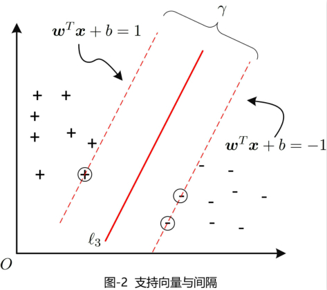
为了增加超平面的鲁棒性,因此需要找到最大间隔的超平面,即
\begin{align}
\max_{(\boldsymbol{w},b)} \ &\frac{1}{||\boldsymbol{w}||}\\
\text{s.t.} \ &y_i(\boldsymbol{w}^T\boldsymbol{x}_i+b)\geq 1 \quad (i=1,\cdots,m)
\end{align}
该问题等价于
\begin{align}
\min_{(\boldsymbol{w},b)} \ & \frac{1}{2}||\boldsymbol{w}||^2\\
\text{s.t.} \ &y_i(\boldsymbol{w}^T\boldsymbol{x}_i+b)\geq 1 \quad (i=1,\cdots,m)
\end{align}
这就是支持向量机(support vector machine, SVM)的基本型。
我们希望找到最大化间隔的超平面
\begin{align}
f(\boldsymbol{x})=\boldsymbol{w}^T\boldsymbol{x}+b
\end{align}
这里我们假设训练样本是线性可分的(上一节中,我们假设样本是两类的)。我们注意到,求解参数$(\boldsymbol{w},b)$本身就是一个凸优化问题,可以通过凸优化工具箱进行计算。另外,我们还可以通过解该问题的对偶问题,来得到最优解。这样所带来的好处是,将一种最优化(最小化)问题转化为另一种最优化(最大化)问题,而后者相对于前者更容易计算。
对于求解标准的优化问题
\begin{align}
\min \ &f_0(\boldsymbol{x})\\
\text{s.t.} \ &f_i(\boldsymbol{x})\leq 0, i=1\cdots,m\\
&h_j(\boldsymbol{x})=0, j=1,\cdots,p
\end{align}
其中$\boldsymbol{x}\in \mathbb{R}^n$。我们假设条件$f_i(\boldsymbol{x})=0$与$h_j(\boldsymbol{x})=0$所构成的定义域集合$\mathcal{D}$是非空的。并且假设$p^{\star}$是最优值。
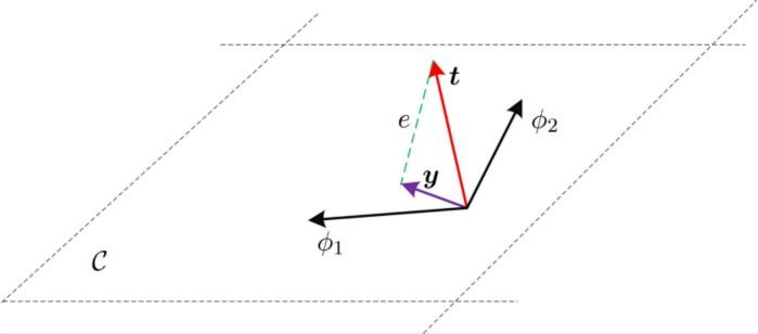
拉个朗日对偶的基本思想,是将该优化问题增广成目标函数$L(\boldsymbol{x},\boldsymbol{\lambda},\boldsymbol{v})$,其中$L$表示映射$L:\mathbb{R}^n\times \mathbb{R}^m\times \mathbb{R}^p\rightarrow \mathbb{R}$。
\begin{align}
L(\boldsymbol{x},\boldsymbol{\lambda},\boldsymbol{v})=f_0(\boldsymbol{x})+\sum\limits_{i=1}^m\lambda_if_i(\boldsymbol{x})+\sum\limits_{i=1}^pv_ih_i(\boldsymbol{x})
\end{align}
定义拉格朗日对偶函数$g:\mathbb{R}^m\times \mathbb{R}^p\rightarrow \mathbb{R}$表示目标函数$L(\boldsymbol{x},\boldsymbol{\lambda},\boldsymbol{v})$关于$\boldsymbol{x}$的下确界
\begin{align}
g(\boldsymbol{\lambda},\boldsymbol{v})=\inf_{\boldsymbol{x}\in \mathcal{D} } L(\boldsymbol{x},\boldsymbol{\lambda},\boldsymbol{v})
\end{align}
此时,通过计算可知$g(\boldsymbol{\lambda},\boldsymbol{v})$是最优值$p^{\star}$的下界
\begin{align}
g(\boldsymbol{\lambda},\boldsymbol{v})\leq p^{\star}
\end{align}
这个结论很容易得到,假设$\tilde{\boldsymbol{x} }\in \mathcal{D}$,对于$\boldsymbol{\lambda}>0$,有
\begin{align}
\sum\limits_{i=1}^m\lambda_if_i(\tilde{\boldsymbol{x} })+\sum\limits_{i=1}^pv_ih_i(\tilde{\boldsymbol{x} })\leq 0
\end{align}
因此,我们可以得到
\begin{align}
L(\tilde{\boldsymbol{x} },\boldsymbol{\lambda},\boldsymbol{v})=f_0(\tilde{\boldsymbol{x} })+\sum\limits_{i=1}^m\lambda_if_i(\tilde{\boldsymbol{x} })+\sum\limits_{i=1}^pv_ih_i(\tilde{\boldsymbol{x} })\leq f_0(\tilde{\boldsymbol{x} })
\end{align}
即
\begin{align}
g(\boldsymbol{\lambda},\boldsymbol{v})=\inf_{\boldsymbol{x}\in \mathcal{D} } L(\boldsymbol{x},\boldsymbol{\lambda},\boldsymbol{v})\leq L(\tilde{\boldsymbol{x} },\boldsymbol{\lambda},\boldsymbol{v})\leq f_0(\tilde{\boldsymbol{x} })
\end{align}
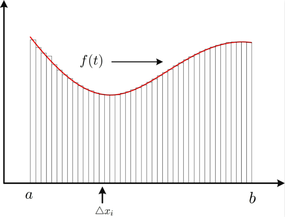
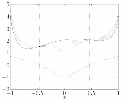
我们通过图3来进行理解。图中,实曲线表示$f_0(\boldsymbol{x})$曲线,虚曲线表示$f_1(\boldsymbol{x})$,由于限制条件$f_1(\boldsymbol{x})\leq 0$,因此$\boldsymbol{x}$的区间为$[-0.46,+0.46]$。显然该定义区间上的最优解为$\boldsymbol{x}^{\star}=-0.46,p^{\star}=1.54$。图中,带点的虚线族表达$L(\lambda,v)$,$\lambda=0.1,0.2,\cdots,1.0$。我们可以看到,$L(\lambda,v)$相对于$p^{\star}$更小。我们需要调整$\lambda$找到使得$L(\lambda,v)$最大的$p^{\star}$的下确界。
利用拉格朗日乘子法,得到目标函数
\begin{align}
L(\boldsymbol{w},b,\boldsymbol{\alpha})=\frac{1}{2}||\boldsymbol{w}||^2+\sum\limits_{i=1}^m\alpha_i(1-y_i(\boldsymbol{w}^T\boldsymbol{x}_i+b))
\end{align}
其中$\alpha_i\geq 0$。令$L(\boldsymbol{w},b,\boldsymbol{\alpha})$对$\boldsymbol{w}$和$b$的偏导数为$0$可得
\begin{align}
\boldsymbol{w}&=\sum\limits_{i=1}^m \alpha_iy_i\boldsymbol{x}_i\\
0&=\sum\limits_{i=1}^m\alpha_iy_i
\end{align}
代入$L(\boldsymbol{w},b,\boldsymbol{\alpha})$中,再考虑约束条件,有
\begin{align}
\max_{\boldsymbol{\alpha} }\ &\sum\limits_{i=1}^m\alpha_i-\frac{1}{2}\sum\limits_{i=1}^m\sum\limits_{j=1}^m \alpha_i\alpha_jy_iy_j\boldsymbol{x}_i^T\boldsymbol{x}_j\\
\text{s.t.}\ & \sum\limits_{i=1}^m\alpha_iy_i=0\\
&\alpha_i\geq 0, \ i=1,\cdots,m
\end{align}
解出$\boldsymbol{\alpha}$之后,即可得到模型
\begin{align}
f(\boldsymbol{x})
&=\boldsymbol{w}^T\boldsymbol{x}+b\\
&=\sum\limits_{i=1}^m\alpha_iy_i\boldsymbol{x}_i^T\boldsymbol{x}+b
\end{align}
由于该过程为拉格朗日对偶得出的解,因此,所得的解,还需满足KKT条件(found in boyd’s convex optimization)。
\begin{align}
\left\{
\begin{matrix}
\alpha_i\geq 0\\
y_if(\boldsymbol{x}_i)-1\geq 0\\
\alpha_i(y_if(\boldsymbol{x}_i)-1)=0
\end{matrix}
\right.
\end{align}
具体求解$\boldsymbol{\alpha}$的过程,是一个二次规划问题,具体方法如SMO(sequential minimal optimization)。SMO方法,每次更新$\boldsymbol{\alpha}$向量中的两个元素(如,$\alpha_i$和$\alpha_j$),固定其余参数。利用$\boldsymbol{\alpha}^T\boldsymbol{y}=0$得到$\alpha_i$和$\alpha_j$的更新。
在之前的内容中,我们假设训练样本是线性可分的。然而实际中,在原始样本空间,可能并不存在这样一个能够完全正确划分两类样本的超平面,比如图4所示“异或”问题,通过将二维平面映射到三维空间,我们可以能够切分样本点的超平面。其中,三维平面按照紫色箭头的方向投影,可以得到原始的异或点。
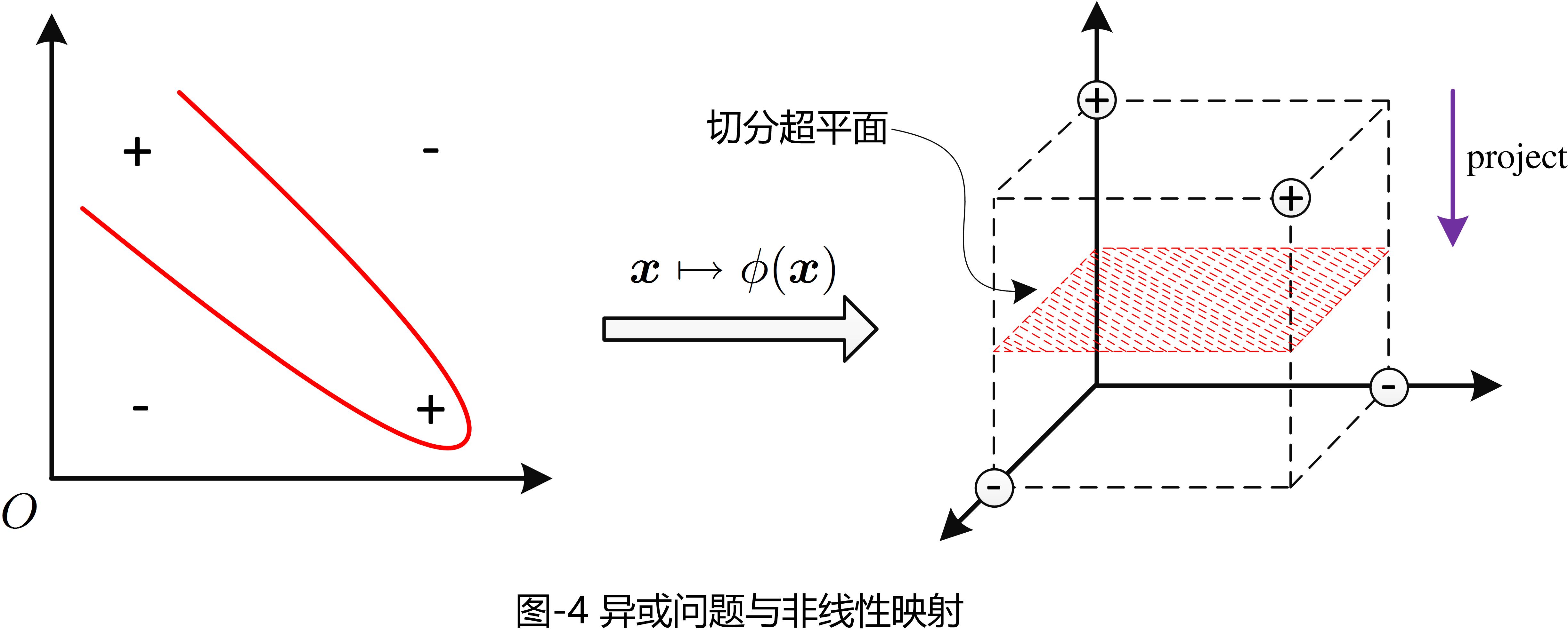
对于这样的问题,通过将样本原始空间映射到高维空间,使得样本在高维空间中线性可分。如果样本空间是有限维的,那么一定存在一个高维空间使得样本可分。我们用$\phi:\mathbb{R}^n\rightarrow \mathbb{R}^p\ (p\gg n)$来表示这样映射,则映射之后的样本表示为$\phi(\boldsymbol{x})$。于是,我们设超平面方程为
\begin{align}
f(\boldsymbol{x})=\boldsymbol{w}^T\phi(\boldsymbol{x})+b
\end{align}
其中$(\boldsymbol{w},b)$是模型参数,类似于上一节知识,参数$(\boldsymbol{w},b)$是如下凸优化问题
\begin{align}
\min\limits_{(\boldsymbol{w},b)}\ &\frac{1}{2}||\boldsymbol{w}||^2\\
\text{s.t.} \ & y_i(\boldsymbol{w}^T\phi(\boldsymbol{x}_i)+b\geq 1)\ i=1,\cdots,m
\end{align}
其对偶问题,为
\begin{align}
\max_{\boldsymbol{\alpha} } \ &\sum\limits_{i=1}^m\alpha_i-\frac{1}{2}\sum\limits_{i=1}\sum\limits_{j=1}\alpha_i\alpha_jy_iy_j\phi(\boldsymbol{x}_i)^T\phi(\boldsymbol{x}_j)\\
\text{s.t.}\ &\sum\limits_{i=1}^m\alpha_iy_i=0\\
&\alpha_i\geq0, \ i=1,\cdots,m
\end{align}
其中$\phi(\boldsymbol{x}_i)^T\phi(\boldsymbol{x}_j)$的计算是非常复杂的,因此我们定义
\begin{align}
\kappa(\boldsymbol{x}_i\boldsymbol{x}_j)=\phi(\boldsymbol{x}_i)^T\phi(\boldsymbol{x}_j)
\end{align}
这里我们称$\kappa(\boldsymbol{x}_i\boldsymbol{x}_j)$为“核函数”。类似于上一节的知识,我们可以得到
\begin{align}
f(\boldsymbol{x})&=\boldsymbol{w}^T\phi(\boldsymbol{x})+b\\
&=\sum_{i=1}^m\alpha_iy_i\kappa(\boldsymbol{x},\boldsymbol{x}_i)+b
\end{align}
该式子表明,模型的最优解可以通过训练样本的核函数展开,这一展开式称为“支持向量展式”(support vecot expansion)
那如何确定核函数或者选择合适的核函数?需要注意的是,在不知道特征映射的形式时,我们并不知道什么样的核函数是合适的,而核函数也仅是隐式地定义了这个特征空间。因此,核函数的选择成为支持向量机最大的变数。常见的核函数有以下几种
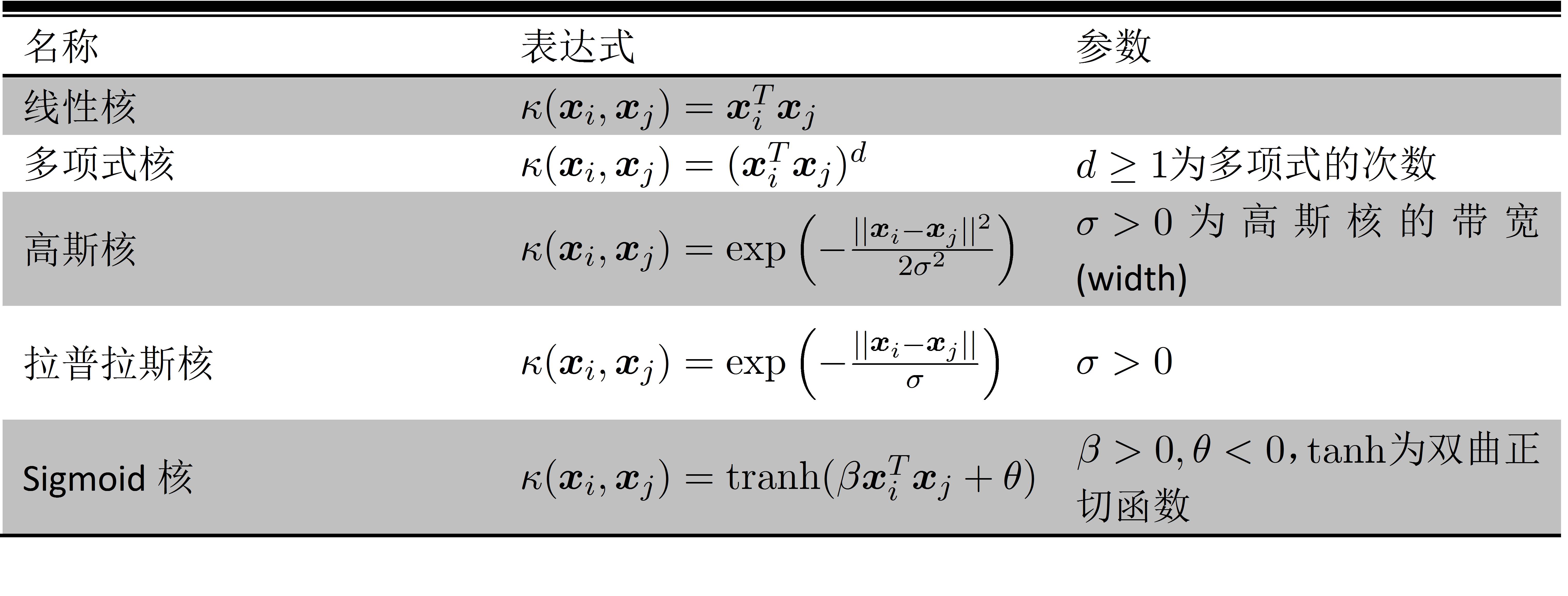
在定义核函数的基础上,人们发展了一系列基于核函数的学习方法,统称为“核方法”(kernel methods)。最常见的,是通过“核化”(即引入核函数)来将线性学习器扩展为非线性学习器,如核线性判别分析(kernelized linear discriminant analysis, KlDA)。
在前面的讨论中,我们假设样本是线性可分的。然而,在现实任务中往往很难确定合适的核函数将训练样本再特征空间中线性可分退一步讲,即使恰好找到某个核函数使训练集在特征空间中线性可分,也很难断定这个貌似线性可分的结果,会不会造成过拟合(即,训练集效果好,测试集效果差)。
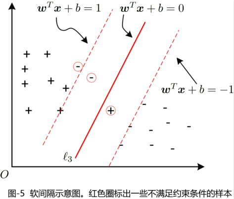
我们通过放松样本线性可分的条件,允许一些支持向量在少数的样本上出错。为此,引入软间隔的概念。如图5所示,这里不做赘述。
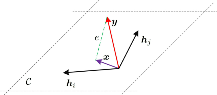
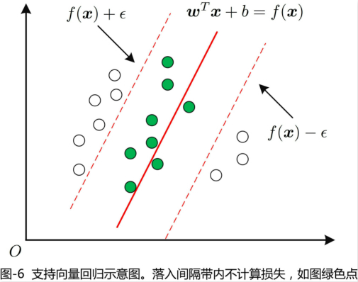
支持向量机所完成的工作是样本分类问题,即,将样本分成两个类,或者三个类。其目的是寻找一个超平面使得样本到超平面的间隔最大。而,支持向量回归,则是通过函数$f(\boldsymbol{x})=\boldsymbol{w}^T\boldsymbol{x}+b$来对样本进行拟合,即我们希望$f(\boldsymbol{x})$与$y$尽可能的靠近。
在回归问题中,我们通常采用模型输出$f(\boldsymbol{x})$和真实输出$y$之间的欧式距离来衡量回归的好坏。当且仅当$f(\boldsymbol{x})$与$y$完全相同,损失才为零。而,支持向量回归(support vector regression, SVR)放松了这个条件,SVR允许$f(\boldsymbol{x})$与$y$之间存在最多为$\epsilon$的误差,这就相当于以$f(\boldsymbol{x})$为中心,构建了如图6的一个宽度为$2\epsilon$的间隔带,若样本落入此间隔带中,则SVR认为是被预测正确的。
于是SVR问题形式化为
\begin{align}
\min_{\boldsymbol{w},b} \ &\frac{1}{2}||\boldsymbol{w}||^2+C\sum\limits_{i=1}^m\ell_{\epsilon} (f(\boldsymbol{x}_i)-y_i) \\
\text{s.t.}\ &f(\boldsymbol{x}_i)-y_i\leq \epsilon\\
&y_i-f(\boldsymbol{x}_i)\leq \epsilon
\end{align}
其中$C(C>0)$是常数,$\ell_{\epsilon}$是不敏感损失函数($\epsilon$-insensitive loss function)。
\begin{align}
\ell_{\epsilon}=\left\{
\begin{matrix}
0 & |z|\leq \epsilon\\
|z|-\epsilon &\text{otherwise}
\end{matrix}
\right.
\end{align}
通过引入松弛变量(或者称,惩罚因子)$\xi_i$和$\hat{\xi}_i$,则该SVR问题重写为
\begin{align}
\min_{\boldsymbol{w},b,\xi_i,\hat{\xi}_i} \ &\frac{1}{2}||\boldsymbol{w}||^2+C\sum_{i=1}^m(\xi_i+\hat{\xi}_i)\\
\text{s.t.}\ &f(\boldsymbol{x}_i)-y_i\leq \epsilon+\xi_i,\\
&y_i-f(\boldsymbol{x}_i)\leq \epsilon+\hat{\xi}_i,\\
&\xi\geq 0,\hat{\xi}_i\geq 0,\ i=1\cdots,m
\end{align}
类似地,我们通过拉格朗日法找到其对偶问题。通过引入拉格朗日乘子$\mu_i\geq 0,\hat{\mu}_i\geq 0,\alpha_i\geq 0,\hat{\alpha}_\geq 0$,由拉格朗日乘子法,可以得到拉格朗日函数
\begin{align}
L(\boldsymbol{w},b,\boldsymbol{\alpha},\hat{\boldsymbol{\alpha} },\boldsymbol{\xi},\hat{\boldsymbol{\xi} },\boldsymbol{\mu},)
&=\frac{1}{2}||\boldsymbol{w}||^2+C\sum\limits_{i=1}^m(\xi_i+\hat{\xi}_i)-\sum\limits_{i=1}^m\mu_i\xi_i-\sum\limits_{i=1}^m\hat{\mu}\hat{\xi}_i\\
&\quad +\sum\limits_{i=1}^m \alpha_i(f(\boldsymbol{x}_i)-y_i-\epsilon-\xi_i)+\sum\limits_{i=1}^m\hat{\alpha}_i (y_i-f(\boldsymbol{x}_i)-\epsilon-\hat{\xi}_i)
\end{align}
令$L(\boldsymbol{w},b,\boldsymbol{\alpha},\hat{\boldsymbol{\alpha} },\boldsymbol{\xi},\hat{\boldsymbol{\xi} },\boldsymbol{\mu},)$对$\boldsymbol{w},b,\xi$和$\hat{\xi}_i$的偏导为$0$,可得
\begin{align}
\boldsymbol{w}&=\sum\limits_{i=1}^m(\hat{\alpha}_i-\alpha_i)\boldsymbol{x}_i\\
0&=\sum\limits_{i=1}^m (\hat{\alpha}_i-\alpha_i)\\
C&=\alpha_i+\mu_i\\
C&=\hat{\alpha}_i+\hat{\mu}_i
\end{align}
代入,可得SVR的对偶问题
\begin{align}
\max_{\boldsymbol{\alpha},\hat{\boldsymbol{\alpha} }} \ & \sum\limits_{i=1}^m y_i(\hat{\alpha}_i-\alpha_i)-\epsilon (\hat{\alpha}_i+\alpha_i)\\
&-\frac{1}{2}\sum_{i=1}^m\sum_{j=1}^m(\hat{\alpha}_i-\alpha_i)(\hat{\alpha}_j-\alpha_j)\boldsymbol{x}_i^T\boldsymbol{x}_j\\
\text{s.t.} \ &\sum_{i=1}^m (\hat{\alpha}_i-\alpha_i)=0,\\
&0\leq \alpha_i,\alpha_j\leq C.
\end{align}
上述过程还需满足KKT条件,即
\begin{align}
\left\{
\begin{matrix}
\alpha_i(f(\boldsymbol{x}_i)-y_i-\epsilon-\xi_i)=0\\
\hat{\alpha}_i(y_i-f(\boldsymbol{x}_i)-\epsilon-\hat{\xi}_i)=0\\
\alpha_i\hat{\alpha}_0=0,\xi_i\hat{\xi}_i=0\\
(C-\alpha_i)\xi_i=0,\ (C-\hat{\alpha}_i)\hat{\xi}_i=0
\end{matrix}
\right.
\end{align}
若解出$\boldsymbol{\alpha}和\hat{\boldsymbol{\alpha} }$,最终可得
\begin{align}
f(\boldsymbol{x})=\sum_{i=1}^m (\hat{\alpha}_i-\alpha_i)\boldsymbol{x}_i^T\boldsymbol{x}+b
\end{align}
其中$b$可以由KKT条件以及$\boldsymbol{\alpha}$和$\hat{\boldsymbol{\alpha} }$得到。
若考虑特征映射$\phi$,即将样本空间映射到更高维的空间,则相应的形式为
\begin{align}
f(\boldsymbol{x})=\sum_{i=1}^m(\hat{\alpha}_i-\alpha_i)\kappa(\boldsymbol{x},\boldsymbol{x}_i)+b
\end{align}
其中$\kappa(\boldsymbol{x}_i,\boldsymbol{x}_j)=\phi(\boldsymbol{x}_i)^T\phi(\boldsymbol{x}_j)$为核函数。
为了理解对信号进行分解的目的,我们先从几何学的角度,回味下平面矢量以及空间矢量的分解。如图1所示,(a)$\overrightarrow{A}=c_1\overrightarrow{v_x}+c_2\overrightarrow{v_y}$,即将平面矢量分解成正交的$x$轴和$y$轴的单位矢量;(b)$\overrightarrow{A}=c_1\overrightarrow{v_x}+c_2\overrightarrow{v_y}+c_3\overrightarrow{v_z}$,即将空间矢量分解成正交的$x$轴、$y$轴和$z$轴的单位矢量。
为此,我们先理清楚什么是矢量正交?
定义:在区间$(t_1,t_2)$上的两个信号$\phi_1(t)$和$\phi_2(t)$,若满足
\begin{align}
\int_{t_1}^{t_2}\phi_1(t)\phi_2(t)=0
\end{align}
则称$\phi_1(t)$和$\phi_2(t)$在区间$(t_1,t_2)$上正交。
正交函数集:如果有$n$个函数$\left\{\phi_1(t),\cdots,\phi_n(t)\right\}$构成一个函数集合,若函数集合在区间$(t_1,t_2)$上满足
\begin{align}
\int_{t_1}^{t_2}\phi_1(t)\phi_2(t)\text{d}t=\left\{
\begin{matrix}
0 &i\ne j\\
K &i=j
\end{matrix}
\right.
\end{align}
其中$K$为常数,则称此函数集为正交函数集。
完备正交函数集:定义集合$\mathcal{S}=\left\{\phi_1(t),\cdots,\phi_n(t)\right\}$是区间$(t_1,t_2)$上的正交函数集,如果除$\mathcal{S}$外,不存在函数$\phi(t)$满足等式
\begin{align}
\int_{t_1}^{t_2} \phi_i(t)\phi(t)=0\quad \forall i=\left\{1,\cdots,n\right\}
\end{align}
则称此函数集为完备正交函数集。我们称该完备集合中的函数$\phi_j(t)$为基或者基底。常见的完备正交函数集合有三角函数集、虚指数函数集。
Example: 证明三角函数集$\left\{1,\cos(nw_0t),\sin(nw_0t)\right\},(n=1,2,\cdots)$是正交函数集合
证:
\begin{align}
\int_{t_0}^{t_0+T}\cos(nw_0t)\cos(mw_0t)\text{d}t&=\left\{
\begin{matrix}
0 &m\ne n\\
\frac{T}{2} &m=n\ne 0\\
T &m=n=0
\end{matrix}
\right.\\
\int_{t_0}^{t_0+T}\sin(nw_0t)\sin(mw_0t)\text{d}t&=\left\{
\begin{matrix}
0 &m\ne n\\
\frac{T}{2} &m=n\ne 0
\end{matrix}
\right.\\
\int_{t_0}^{t_0+T}\sin(nw_0t)\cos(mw_0t)\text{d}t&=0
\end{align}
因此三角函数集为正交函数集。
【注】如果函数$f(t)$是周期为$T$的周期信号,则有$\int_{a}^{T+a}f(t)\text{d}t=\int_{0}^{T}f(t)\text{d}t$。
设$n$个函数$\phi_1(t),\cdots,\phi_n(t)$在区间$(t_1,t_2)$构成一个正交函数集$\mathcal{S}$。将任意信号$f(t)$表示成这$n$个函数的线性组合来近似,可表示为
\begin{align}
f(t)\approx a_1\phi_1(t)+\cdots a_n\phi_n(t)=\sum\limits_{i=1}^na_i\phi_i(t)
\end{align}
为此,我们需要确定$a_i (i=1,\cdots n)$的具体取值,来确保$\sum\limits_{i=1}^na_i\phi_i(t)$是对$f(t)$的最佳近似。我们选取均方误差(mean square error, MSE)来衡量这个近似的效果
\begin{align}
\text{MSE}=\frac{1}{t_2-t_1}\int_{t_1}^{t_2}\left(f(t)-\sum\limits_{i=1}^na_i\phi_i(t)\right)^2\text{d}t
\end{align}
为使得MSE最小,计算MSE对$a_j$的偏导如下
\begin{align}
\frac{\partial \text{MSE} }{\partial a_j}
&=\frac{1}{t_2-t_1}\frac{\partial }{\partial a_j}\int_{t_1}^{t_2}\left(f(t)-\sum\limits_{i=1}^na_i\phi_i(t)\right)^2\text{d}t\\
&\overset{(a)}{=}\frac{1}{t_2-t_1}\int_{t_1}^{t_2}\frac{\partial }{\partial a_j}\left(f(t)-\sum\limits_{i=1}^na_i\phi_i(t)\right)^2\text{d}t\\
&=-\frac{1}{t_2-t_1}\int_{t_1}^{t_2}2\left(f(t)-\sum\limits_{i=1}^na_i\phi_i(t)\right)\phi_j(t)\text{d}t\\
&\overset{(b)}{=}\frac{2a_j}{t_2-t_1}\int_{t_1}^{t_2}\phi_j^2(t)\text{d}t-\frac{2}{t_2-t_1}\int_{t_1}^{t_2}f(t)\phi_j(t)\text{d}t
\end{align}
其中步骤$(a)$成立,假设被积函数性质足够好,使得积分和偏导顺序可以交换;步骤$(b)$成立,利用完备正交函数集合,函数正交的性质。令偏导数为零,得到
\begin{align}
a_j=\frac{\int_{t_1}^{t_2}f(t)\phi_j(t)\text{d}t}{\int_{t_1}^{t_2}\phi_j^2(t)\text{d}t} \quad i=(1,\cdots,n)
\end{align}
定义$K_j=\int_{t_1}^{t_2}\phi_j^2(t)\text{d}t$,则参数$a_j$可以表示为
\begin{align}
a_j=\frac{1}{K_j}\int_{t_1}^{t_2}f(t)\phi_j(t)\text{d}t
\end{align}
到这里,我们会发现,信号的正交分解,跟矢量投影很相似。将矢量$\overrightarrow{A}$投影到矢量$\overrightarrow{a}$上,其投影长度$\frac{\overrightarrow{A}\cdot \overrightarrow{a} }{|\overrightarrow{a}|}$。注意这里所得到的$a_j$表达式是基于均方误差最小准则得到的,均方误差刻画的是真实值和近似值的欧式距离,根据不同的规则,可以得到不同的解。
根据上一节知识,我们尝试将信号$f(t)$分解到三角函数集$\mathcal{S}=\left\{1,\cos(nw_0t),\sin(nw_0t)\right\},(n=1,\cdots)$上,即将$f(t)$表示成该集合中基的线性组合,如下
\begin{align}
f(t)=\frac{a_0}{2}+\sum\limits_{n=1}^{+\infty}a_n\cos(nw_0t)+\sum\limits_{n=1}^{+\infty}b_n\sin (nw_0t)
\end{align}
为了计算$a_n$
合并同频率的$\cos(nw_0t),\sin(nw_0t)$,如下
\begin{align}
f(t)=\frac{A_0}{2}+\sum\limits_{n=1}^{+\infty}A_n \cos(nw_0t+\psi_n)
\end{align}
其中
\begin{align}
\left\{
\begin{matrix}
A_0=a_0\qquad \quad \quad \quad\\
A_n=\sqrt{a_n^2+b_n^2}\quad \quad\\
\psi_n=-\arctan (\frac{b_n}{a_n})
\end{matrix}
\right.
\end{align}
傅里叶级数是对周期信号的最佳近似,做这种近似的目的就是为了方便计算和分析信号,但是在实际信号分析中,使用三角级数计算比较麻烦。因此通过欧拉公式将傅里叶级数的三角形式转换成指数形式。
\begin{align}
\cos(t)=\frac{e^{jt}+e^{-jt} }{2}
\end{align}
应用欧拉公式,信号$f(t)$表示为
\begin{align}
f(t)&=\frac{A_0}{2}+\sum\limits_{n=1}^{+\infty}\frac{A_n}{2}\left(e^{j(nw_0t+\psi_n)}+e^{-j(nw_0t+\psi_n)}\right)\\
&=\frac{A_0}{2}+\sum\limits_{n=1}^{+\infty}\frac{A_n}{2}e^{j(nw_0t+\psi_n)}+\sum\limits_{n=1}^{+\infty}\frac{A_n}{2}e^{-j(nw_0t+\psi_n)}\\
&=\frac{A_0}{2}+\sum\limits_{n=1}^{+\infty}\frac{A_n}{2}e^{j(nw_0t+\psi_n)}+\sum\limits_{n=-1}^{-\infty}\frac{A_{-n} }{2}e^{jnw_0t}e^{-j\psi_{-n} }
\end{align}
由于$A_n=\sqrt{a_n^2+b_n^2}$是关于$n$的偶函数,$\psi_n$是关于$n$的奇函数,因此有
\begin{align}
f(t)=\frac{A_0}{2}+\sum\limits_{n=1}^{+\infty}\frac{A_n}{2}e^{j(nw_0t+\psi_n)}+\sum\limits_{n=-1}^{-\infty}\frac{A_n}{2}e^{j(nw_0t+\psi_n)}
\end{align}
令$A_n|_{n=0}=A_0$,因此有
\begin{align}
f(t)=\sum\limits_{n=-\infty}^{+\infty}\frac{A_n}{2}e^{j\psi_n}e^{jnw_0t}
\end{align}
令$F_n=\frac{A_n}{2}e^{j\psi_n}$,即得到信号的傅里叶级数的虚指数形式的表达式
\begin{align}
f(t)=\sum\limits_{n=-\infty}^{+\infty}F_ne^{jnw_0t}
\end{align}
类似地,这里$F_n$的表达式也可以利用信号正交或者均方误差最小的方式来求解,得到
\begin{align}
F_n=\frac{1}{T}\int_T f(t)e^{-jnw_0t}\text{d}t
\end{align}